Data wrangling I & II

Quantitative Methods for
International Politics

IPOL 3270 • Fall 2026

September 13, 2026

Plan for today

Manipulating data with {dplyr}
filter()
select()
arrange()
mutate()
Multiple verbs and pipes
summarise()
group_by()

Manipulating data with {dplyr}

Your turn #0: Load data

Run the setup chunk
Take a look at the gapminder data

The `gapminder` data

gapminder

# A tibble: 1,704 × 6
   country     continent  year lifeExp      pop gdpPercap
   <fct>       <fct>     <int>   <dbl>    <int>     <dbl>
 1 Afghanistan Asia       1952    28.8  8425333      779.
 2 Afghanistan Asia       1957    30.3  9240934      821.
 3 Afghanistan Asia       1962    32.0 10267083      853.
 4 Afghanistan Asia       1967    34.0 11537966      836.
 5 Afghanistan Asia       1972    36.1 13079460      740.
 6 Afghanistan Asia       1977    38.4 14880372      786.
 7 Afghanistan Asia       1982    39.9 12881816      978.
 8 Afghanistan Asia       1987    40.8 13867957      852.
 9 Afghanistan Asia       1992    41.7 16317921      649.
10 Afghanistan Asia       1997    41.8 22227415      635.
# ℹ 1,694 more rows

The tidyverse

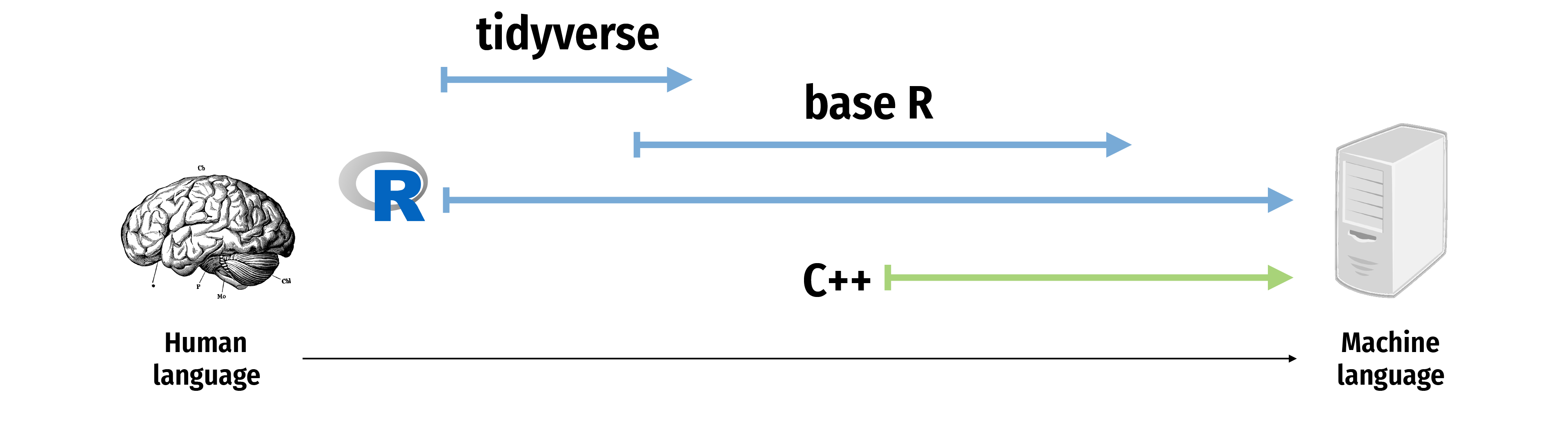
The tidyverse

{dplyr}: verbs for data

Extract rows with `filter()`
Extract columns with `select()`
Arrange/sort rows with `arrange()`
Make new columns with `mutate()`
Make group summaries with `group_by() \|> summarise()`

`filter()`

Extract rows that meet some sort of test

filter(
  DATA, 
  ...
)

DATA = Data frame to transform
... = One or more tests (filter() returns each row for which the test is TRUE)

filter(gapminder, country == "Egypt")

country	continent	year
Afghanistan	Asia	1952
Afghanistan	Asia	1957
Afghanistan	Asia	1962
Afghanistan	Asia	1967
Afghanistan	Asia	1972
…	…	…

country	continent	year
Egypt	Africa	1952
Egypt	Africa	1957
Egypt	Africa	1962
Egypt	Africa	1967
Egypt	Africa	1972
Egypt	Africa	1977

Assignment

What’s the difference here?

filter(gapminder, country == "Egypt")

data_egypt <- filter(gapminder, country == "Egypt")

`<-`

<- assigns the output from the righthand side to an object with the name on the lefthand side

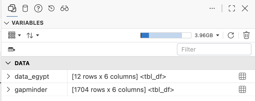
data_egypt <- filter(gapminder, country == "Egypt")

`filter()`

filter(
  gapminder,
  country == "Egypt"
)

One = sets an argument

Two == tests if equal (returns TRUE or FALSE)

Logical tests

Test	Meaning	Test	Meaning
`x < y`	Less than	`x %in% y`	In (group membership)
`x > y`	Greater than	`is.na(x)`	Is missing
`x == y`	Equal to	`!is.na(x)`	Is not missing
`x <= y`	Less than or equal to
`x >= y`	Greater than or equal to
`x != y`	Not equal to

Your turn #1: Filtering

Use filter() and logical tests to show…

The data for Canada
All data for countries in Oceania
Rows where the life expectancy is greater than 82

filter(gapminder, country == "Canada")

filter(gapminder, continent == "Oceania")

filter(gapminder, lifeExp > 82)

Common mistakes

Using = instead of ==

filter(
  gapminder,
  country = "Canada"
)

filter(
  gapminder,
  country == "Canada"
)

Quote use

filter(
  gapminder,
  country == Canada
)

filter(
  gapminder,
  country == "Canada"
)

`filter()` with multiple conditions

Extract rows that meet every test

filter(gapminder, country == "Egypt", year > 2000)

`filter()` with multiple conditions

filter(gapminder, country == "Egypt", year > 2000)

country	continent	year
Afghanistan	Asia	1952
Afghanistan	Asia	1957
Afghanistan	Asia	1962
Afghanistan	Asia	1967
Afghanistan	Asia	1972
…	…	…

country	continent	year
Egypt	Africa	2002
Egypt	Africa	2007

Boolean operators

Operator	Meaning
`a & b`	and
`a \| b`	or
`!a`	not

Default is “and”

These do the same thing:

filter(gapminder, country == "Egypt", year > 2000)

filter(gapminder, country == "Egypt" & year > 2000)

Your turn #2: Filtering

Use filter() and Boolean logical tests to show…

Canada before 1970
Countries where life expectancy in 2007 is below 50
Countries where life expectancy in 2007 is below 50 and are not in Africa

filter(gapminder, country == "Canada", year < 1970)

filter(gapminder, year == 2007, lifeExp < 50)

filter(
  gapminder,
  year == 2007,
  lifeExp < 50,
  continent != "Africa"
)

Common mistakes

Collapsing multiple tests into one

filter(
  gapminder,
  1960 < year < 1980
)

filter(
  gapminder,
  year > 1960, year < 1980
)

Common mistakes

Using multiple tests instead of %in%

filter(
  gapminder,
  country == "Mexico" | country == "Canada" | 
    country == "United States"
)

filter(
  gapminder,
  country %in% c("Mexico", "Canada", "United States")
)

Common syntax

Every {dplyr} verb function follows the same pattern!

VERB(DATA, ...)

VERB = {dplyr} function/verb
DATA = Data frame to transform
... = Stuff the verb does

`select()`

Keep specific columns

select(
  DATA, 
  ...
)

DATA = Data frame to work with
... = Columns

select(gapminder, year, country)

country	continent	year
Afghanistan	Asia	1952
Afghanistan	Asia	1957
Afghanistan	Asia	1962
Afghanistan	Asia	1967
Afghanistan	Asia	1972
…	…	…

year	country
1952	Afghanistan
1957	Afghanistan
1962	Afghanistan
1967	Afghanistan
1972	Afghanistan
…	…

Remove columns with `-`

select(gapminder, -continent)

country	year	lifeExp	pop	gdpPercap
Afghanistan	1952	28.801	8425333	779.4453145
Afghanistan	1957	30.332	9240934	820.8530296
Afghanistan	1962	31.997	10267083	853.10071
Afghanistan	1967	34.02	11537966	836.1971382
Afghanistan	1972	36.088	13079460	739.9811058
…	…	…	…	…

Keep other columns with `everything()`

select(gapminder, year, pop, everything())

year	pop	country	continent	lifeExp	gdpPercap
1952	8425333	Afghanistan	Asia	28.801	779.4453145
1957	9240934	Afghanistan	Asia	30.332	820.8530296
1962	10267083	Afghanistan	Asia	31.997	853.10071
1967	11537966	Afghanistan	Asia	34.02	836.1971382
1972	13079460	Afghanistan	Asia	36.088	739.9811058
…	…	…	…	…	…

Helper functions

select(gapminder, starts_with("c"))

country	continent
Afghanistan	Asia
Afghanistan	Asia
Afghanistan	Asia
Afghanistan	Asia
Afghanistan	Asia
…	…

Helper functions

Operator	Meaning
`starts_with()`	Starts with an exact prefix
`ends_with()`	Ends with an exact suffix
`contains()`	Contains some text
`matches()`	Matches a search
`num_range()`	Contains a range of numbers

Your turn #3: Selecting

Use select() to…

Remove the gdpPercap column
Make year be the first column and keep all the others
Keep all the columns that end with “p”

select(gapminder, -gdpPercap)

select(gapminder, year, everything())

select(gapminder, ends_with("p"))

`arrange()`

Sort rows by specific columns

arrange(
  DATA, 
  ...
)

DATA = Data frame to sort
... = Columns

arrange(gapminder, lifeExp)

country	year	lifeExp
Afghanistan	1952	28.801
Afghanistan	1957	30.332
Afghanistan	1962	31.997
Afghanistan	1967	34.02
Afghanistan	1972	36.088
…	…	…

country	year	lifeExp
Rwanda	1992	23.599
Afghanistan	1952	28.801
Gambia	1952	30
Angola	1952	30.015
Sierra Leone	1952	30.331
…	…	…

Go the other way with `desc()`

arrange(gapminder, desc(lifeExp))

country	year	lifeExp
Afghanistan	1952	28.801
Afghanistan	1957	30.332
Afghanistan	1962	31.997
Afghanistan	1967	34.02
Afghanistan	1972	36.088
…	…	…

country	year	lifeExp
Japan	2007	82.603
Hong Kong, China	2007	82.208
Japan	2002	82
Iceland	2007	81.757
Switzerland	2007	81.701
…	…	…

Sort by multiple columns

arrange(gapminder, desc(year), lifeExp)

country	year	lifeExp
Afghanistan	1952	28.801
Afghanistan	1957	30.332
Afghanistan	1962	31.997
Afghanistan	1967	34.02
Afghanistan	1972	36.088
…	…	…

country	year	lifeExp
Swaziland	2007	39.613
Mozambique	2007	42.082
Zambia	2007	42.384
Sierra Leone	2007	42.568
Lesotho	2007	42.592
…	…	…

Your turn #4: Arranging

Use arrange() to…

Sort the data so that the countries with the highest GDP per capita are at the top
Sort the data so that the countries with the lowest population are at the top, starting in the earliest year
Sort the data so that the countries with the lowest population are at the top, starting in the latest year

arrange(gapminder, desc(gdpPercap))

arrange(gapminder, year, pop)

arrange(gapminder, desc(year), pop)

How can we remember all this??!

You can’t! It’ll come with practice.

Copy/paste/tweak

Your own problem sets
R’s help
ModernDive (i.e. actually do the readings 😀)
R Primers from the readings
Posit Cheatsheets

`mutate()`

Create new columns

mutate(
  DATA, 
  ...
)

DATA = Data frame to transform
... = Columns

mutate(gapminder, gdp = gdpPercap * pop)

country	year	gdpPercap	pop
Afghanistan	1952	779	8,425,333
Afghanistan	1957	821	9,240,934
Afghanistan	1962	853	10,267,083
Afghanistan	1967	836	11,537,966
Afghanistan	1972	740	13,079,460
…	…	…	…

country	year	…	gdp
Afghanistan	1952	…	6,567,086,330
Afghanistan	1957	…	7,585,448,670
Afghanistan	1962	…	8,758,855,797
Afghanistan	1967	…	9,648,014,150
Afghanistan	1972	…	9,678,553,274
Afghanistan	1977	…	11,697,659,231

mutate(
  gapminder,
  gdp = gdpPercap * pop,
  pop_mil = round(pop / 1000000)
)

country	year	gdpPercap	pop
Afghanistan	1952	779	8,425,333
Afghanistan	1957	821	9,240,934
Afghanistan	1962	853	10,267,083
Afghanistan	1967	836	11,537,966
Afghanistan	1972	740	13,079,460
…	…	…	…

country	year	…	gdp	pop_mil
Afghanistan	1952	…	6,567,086,330	8
Afghanistan	1957	…	7,585,448,670	9
Afghanistan	1962	…	8,758,855,797	10
Afghanistan	1967	…	9,648,014,150	12
Afghanistan	1972	…	9,678,553,274	13
Afghanistan	1977	…	11,697,659,231	15

`ifelse()`

Do conditional tests within mutate()

ifelse(
  TEST,
  VALUE_IF_TRUE,
  VALUE_IF_FALSE
)

TEST = A logical test
VALUE_IF_TRUE = What happens if test is true
VALUE_IF_FALSE = What happens if test is false

mutate(
  gapminder,
  after_1960 = ifelse(year > 1960, TRUE, FALSE)
)

mutate(
  gapminder,
  after_1960 = ifelse(
    year > 1960,
    "After 1960",
    "Before 1960"
  )
)

Your turn #5: Mutating

Use mutate() to…

Add an africa column that is TRUE if the country is on the African continent
Add a column for logged GDP per capita (hint: use log())
Add an africa_asia column that says “Africa or Asia” if the country is in Africa or Asia, and “Not Africa or Asia” if it’s not

mutate(
  gapminder,
  africa = ifelse(continent == "Africa", TRUE, FALSE)
)

mutate(gapminder, log_gdpPercap = log(gdpPercap))

mutate(
  gapminder,
  africa_asia = ifelse(
    continent %in% c("Africa", "Asia"),
    "Africa or Asia",
    "Not Africa or Asia"
  )
)

`rename()`

Rename existing columns

rename(
  DATA, 
  ...
)

DATA = Data frame to transform
... = new = old

rename(
  gapminder,
  life_expectancy = lifeExp,
  gdp_per_capita = gdpPercap
)

Legal column names

Columns in R can be whatever you want…

rename(gapminder, blah = lifeExp, bloop = gdpPercap)

…EXCEPT (1) they can’t start with numbers and (2) they can’t have spaces

Use backticks (`s) to work with “illegal” column names

rename(
  gapminder,
  `Life Expectancy` = lifeExp,
  `1234` = gdpPercap
)

Multiple verbs and pipes

What if you have multiple verbs?

Make a dataset for just 2002 and calculate logged GDP per capita

Approach 1: Intermediate variables

gapminder_2002 <- filter(gapminder, year == 2002)

gapminder_2002_log <- mutate(
  gapminder_2002,
  log_gdpPercap = log(gdpPercap)
)

What if you have multiple verbs?

Make a dataset for just 2002 and calculate logged GDP per capita

Approach 2: Nested functions

gapminder_2002_log <- filter(
  mutate(
    gapminder,
    log_gdpPercap = log(gdpPercap)
  ),
  year == 2002)

What if you have multiple verbs?

Make a dataset for just 2002 and calculate logged GDP per capita

Approach 3: Pipes!

The |> operator (pipe) takes an object on the left and passes it as the first argument of the function on the right

gapminder |> filter(_____, country == "Canada")

What if you have multiple verbs?

These do the same thing!

filter(gapminder, country == "Canada")

gapminder |> filter(country == "Canada")

What if you have multiple verbs?

Make a dataset for just 2002 and calculate logged GDP per capita

Approach 3: Pipes!

gapminder_2002_log <- gapminder |>
  filter(year == 2002) |>
  mutate(log_gdpPercap = log(gdpPercap))

`|>`

leave_house(
  get_dressed(
    get_out_of_bed(
      wake_up(me, time = "8:00"), 
      side = "correct"), 
    pants = TRUE, shirt = TRUE), 
  car = TRUE, bike = FALSE
)

me |>
  wake_up(time = "8:00") |>
  get_out_of_bed(side = "correct") |>
  get_dressed(pants = TRUE, shirt = TRUE) |>
  leave_house(car = TRUE, bike = FALSE)

`|>` vs `%>%`

There are actually multiple pipes

%>% was invented first, but requires a package to use
|> is part of base R

They’re interchangeable 99% of the time

(Just be consistent)

`summarise()`

Compute a table of summaries

gapminder |>
  summarise(mean_life = mean(lifeExp))

country	continent	year	lifeExp
Afghanistan	Asia	1952	28.801
Afghanistan	Asia	1957	30.332
Afghanistan	Asia	1962	31.997
Afghanistan	Asia	1967	34.02
…	…	…	…

mean_life
59.47444

`summarise()`

gapminder |>
  summarise(
    mean_life = mean(lifeExp),
    min_life = min(lifeExp)
  )

country	continent	year	lifeExp
Afghanistan	Asia	1952	28.801
Afghanistan	Asia	1957	30.332
Afghanistan	Asia	1962	31.997
Afghanistan	Asia	1967	34.02
Afghanistan	Asia	1972	36.088
…	…	…	…

mean_life	min_life
59.47444	23.599

Your turn #6: Summarizing

Use summarise() to calculate…

The first (minimum) year in the dataset
The last (maximum) year in the dataset
The number of rows in the dataset (use the cheatsheet)
The number of distinct countries in the dataset (use the cheatsheet)

gapminder |>
  summarise(
    first = min(year),
    last = max(year),
    num_rows = n(),
    num_unique = n_distinct(country)
  )

first	last	num_rows	num_unique
1952	2007	1704	142

Your turn #7: Summarizing

Use filter() and summarise() to calculate (1) the number of unique countries and (2) the median life expectancy in Africa in 2007

gapminder |>
  filter(continent == "Africa", year == 2007) |>
  summarise(
    n_countries = n_distinct(country),
    med_le = median(lifeExp)
  )

n_countries	med_le
52	52.9265

`group_by()`

Put rows into groups based on values in a column

gapminder |> group_by(continent)

Nothing happens by itself!

Powerful when combined with summarise()

`group_by() |> summarise()`

gapminder |>
  group_by(continent) |>
  summarise(
    n_countries = n_distinct(country),
    avg_life_exp = mean(lifeExp)
  )

continent	n_countries	avg_life_exp
Africa	52	48.86533
Americas	25	64.65874
Asia	33	60.06490
Europe	30	71.90369
Oceania	2	74.32621

pollution |> 
  summarise(
    mean = mean(amount), sum = sum(amount), n = n()
  )

city	particle_size	amount
New York	Large	23
New York	Small	14
London	Large	22
London	Small	16
Beijing	Large	121
Beijing	Small	56

mean	sum	n
42	252	6

pollution |>
  group_by(city) |>
  summarise(
    mean = mean(amount), sum = sum(amount), n = n()
  )

city	particle_size	amount
New York	Large	23
New York	Small	14
London	Large	22
London	Small	16
Beijing	Large	121
Beijing	Small	56

city	mean	sum	n
Beijing	88.5	177	2
London	19.0	38	2
New York	18.5	37	2

pollution |>
  group_by(particle_size) |>
  summarise(
    mean = mean(amount), sum = sum(amount), n = n()
  )

city	particle_size	amount
New York	Large	23
New York	Small	14
London	Large	22
London	Small	16
Beijing	Large	121
Beijing	Small	56

particle_size	mean	sum	n
Large	55.33333	166	3
Small	28.66667	86	3

Your turn #8: Grouping and summarizing

Find the minimum, maximum, and median life expectancy for each continent

Find the minimum, maximum, and median life expectancy for each continent in 2007 only

gapminder |>
  group_by(continent) |>
  summarise(
    min_le = min(lifeExp),
    max_le = max(lifeExp),
    med_le = median(lifeExp)
  )

gapminder |>
  filter(year == 2007) |>
  group_by(continent) |>
  summarise(
    min_le = min(lifeExp),
    max_le = max(lifeExp),
    med_le = median(lifeExp)
  )

Data wrangling I & II

Plan for today

Manipulating data with {dplyr}

Your turn #0: Load data

The gapminder data

The tidyverse

The tidyverse

{dplyr}: verbs for data

filter()

filter()

Assignment

<-

filter()

Logical tests

Your turn #1: Filtering

Common mistakes

filter() with multiple conditions

filter() with multiple conditions

Boolean operators

Default is “and”

Your turn #2: Filtering

Common mistakes

Common mistakes

Common syntax

select()

select()

Remove columns with -

Keep other columns with everything()

Helper functions

Helper functions

Your turn #3: Selecting

arrange()

arrange()

Go the other way with desc()

Sort by multiple columns

Your turn #4: Arranging

How can we remember all this??!

mutate()

mutate()

ifelse()

Your turn #5: Mutating

rename()

Legal column names

Multiple verbs and pipes

What if you have multiple verbs?

Approach 1: Intermediate variables

What if you have multiple verbs?

Approach 2: Nested functions

What if you have multiple verbs?

Approach 3: Pipes!

What if you have multiple verbs?

What if you have multiple verbs?

Approach 3: Pipes!

|>

|> vs %>%

summarise()

summarise()

summarise()

Your turn #6: Summarizing

Your turn #7: Summarizing

group_by()

group_by()

group_by() |> summarise()

Your turn #8: Grouping and summarizing

The `gapminder` data

`filter()`

`filter()`

`<-`

`filter()`

`filter()` with multiple conditions

`filter()` with multiple conditions

`select()`

`select()`

Remove columns with `-`

Keep other columns with `everything()`

`arrange()`

`arrange()`

Go the other way with `desc()`

`mutate()`

`mutate()`

`ifelse()`

`rename()`

`|>`

`|>` vs `%>%`

`summarise()`

`summarise()`

`summarise()`

`group_by()`

`group_by()`

`group_by() |> summarise()`