Data importing and tidy data II
Quantitative Methods for
International Politics
IPOL 3270 • Fall 2026
September 22, 2026

Plan for today
Downloading, making,
and reading data
Tidy data
Pivoting data
Downloading, making, and reading data
What does data look like?
Rectangles!
- CSV files (
.csv) - Excel files (
.xlsx) - Google Sheets
- Other programs like Stata (
.dta)
CSV files
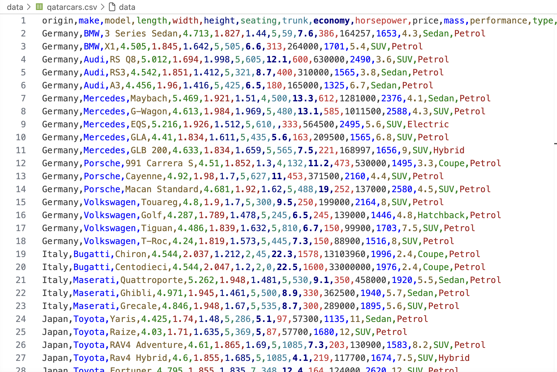
CSV files
Excel files
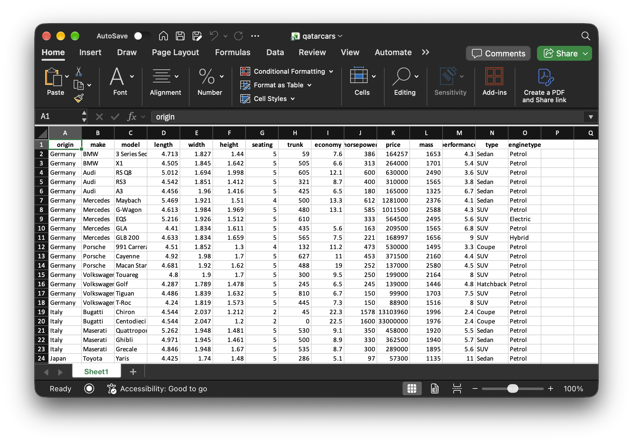
Excel files
Google Sheets
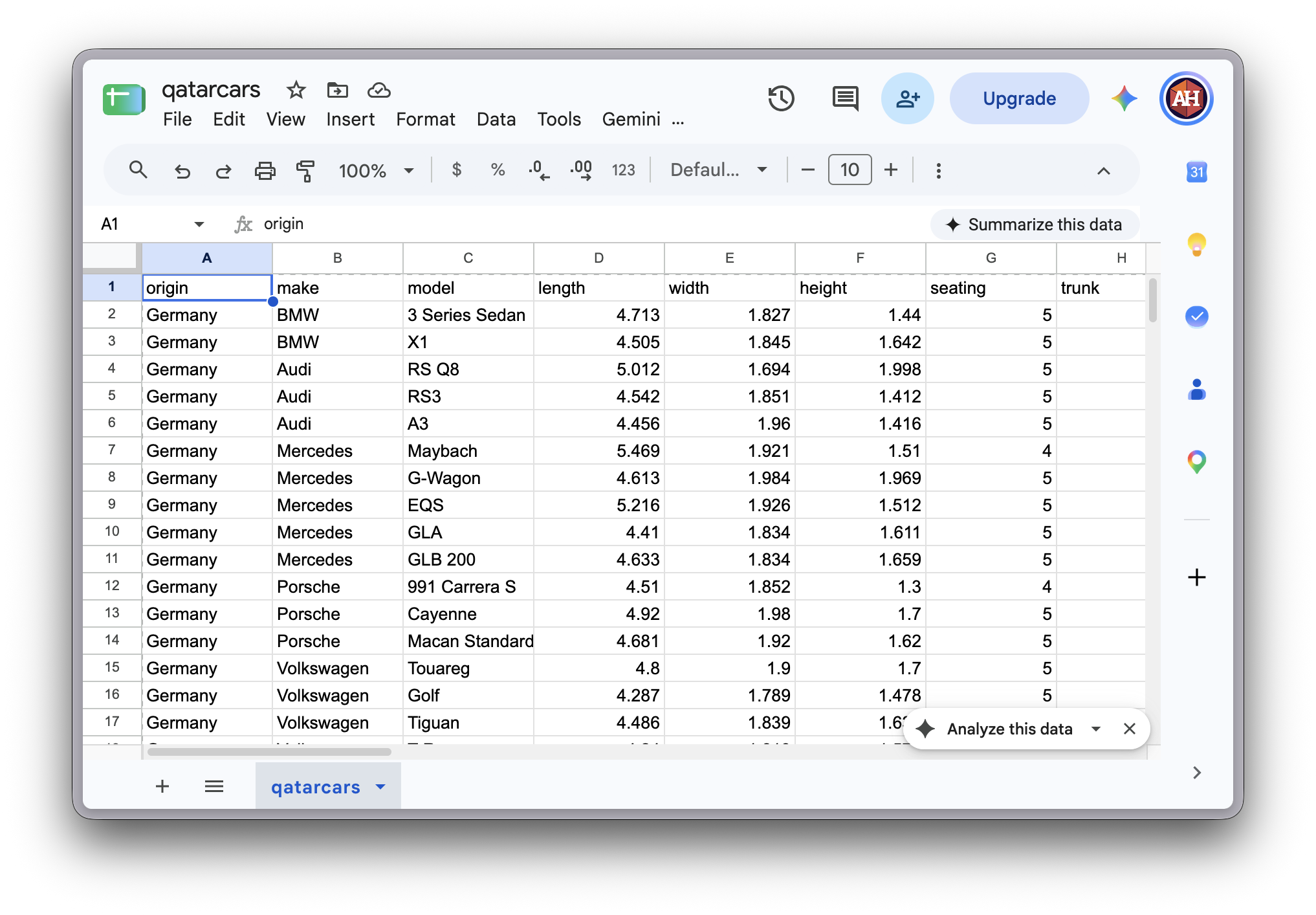
Google Sheets
(Though often easier to just download as CSV)
Other programs (Stata, SAS, SPSS)
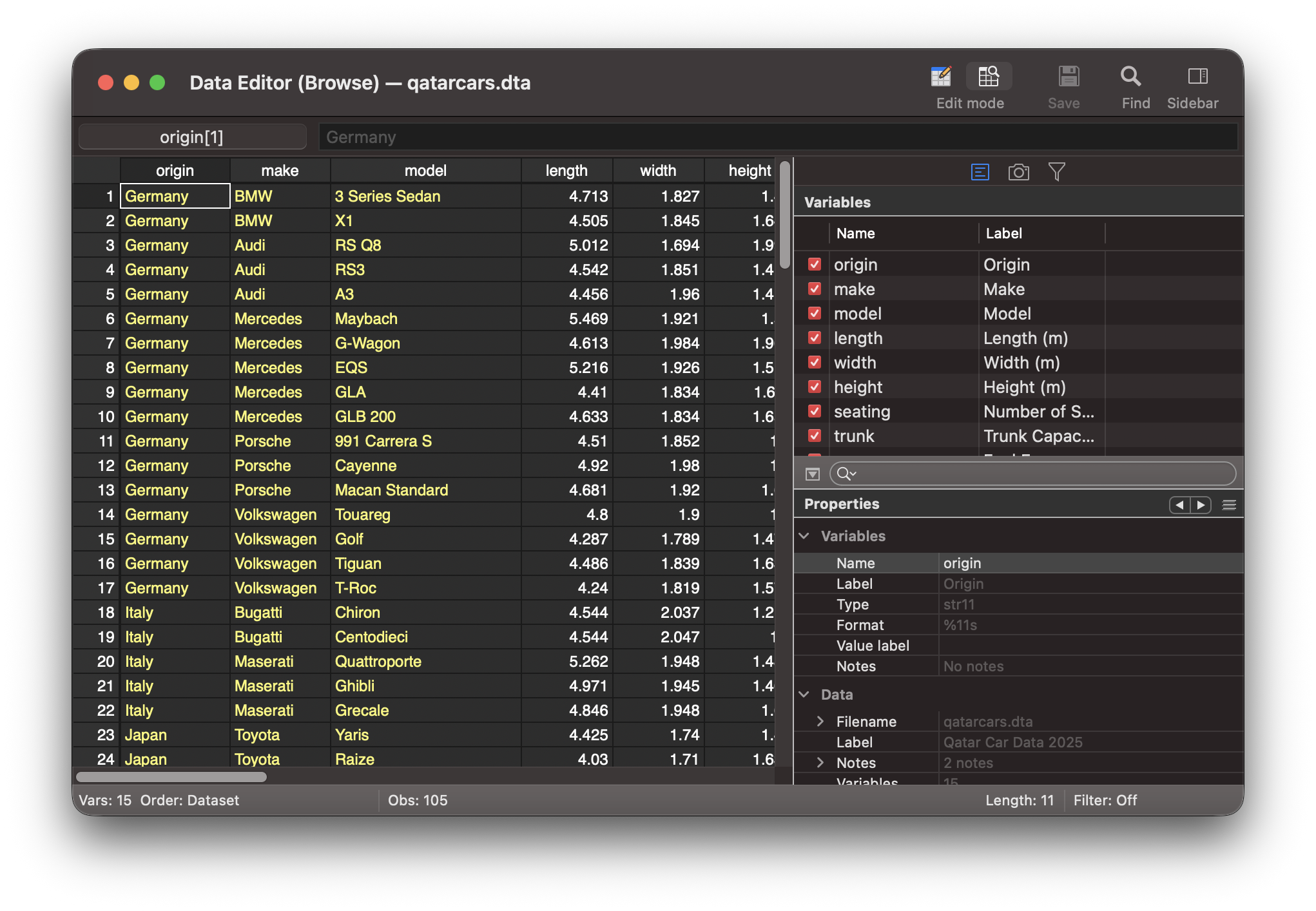
Other programs (Stata, SAS, SPSS)
Let Positron help you!
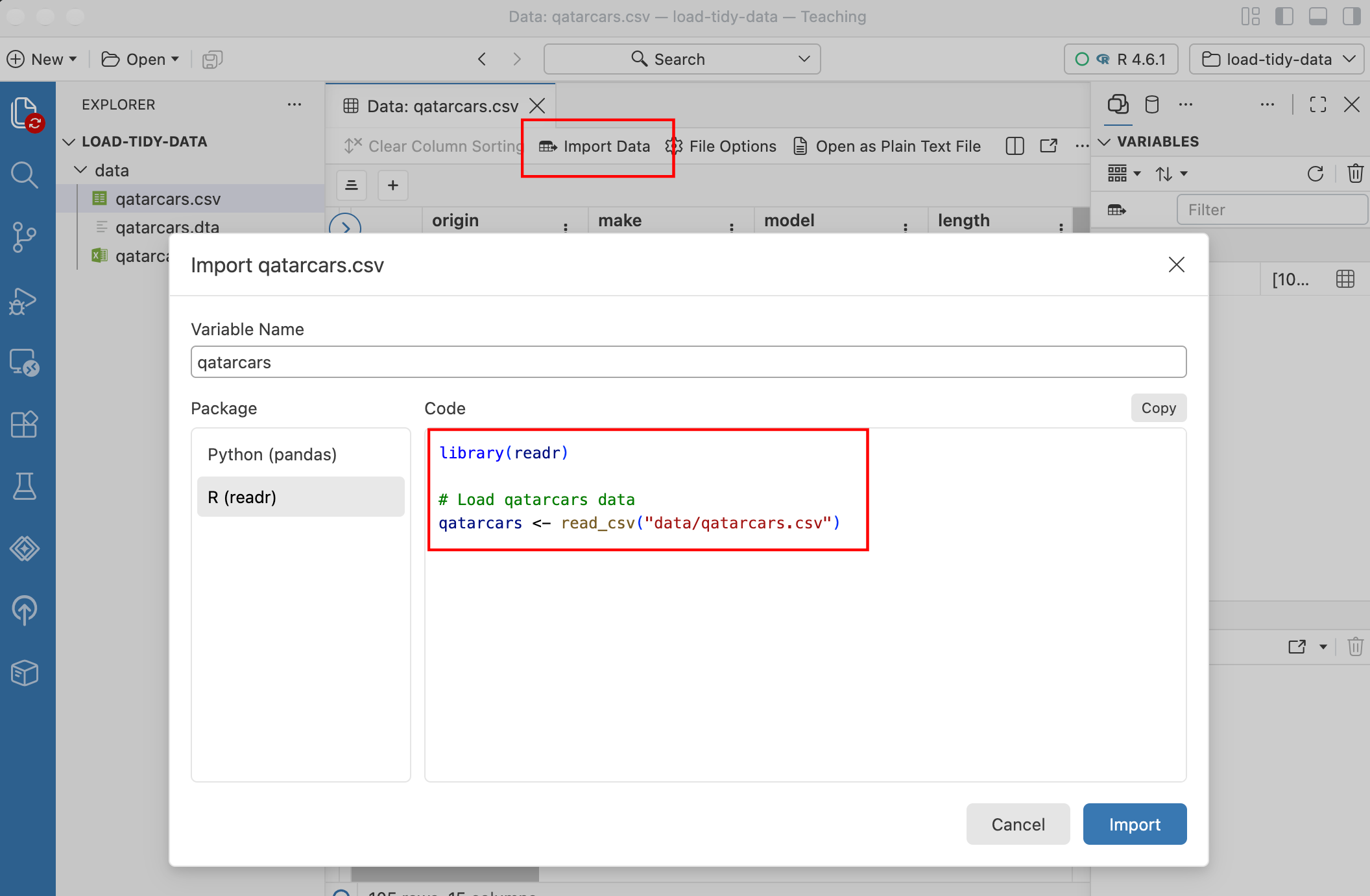
Your/our turn #0
- Create a new empty Positron project!
- Download the
example-data.zipfolder from the class website, unzip it, and put it in your project
Your turn #1
- Download a dataset from Qatar’s Open Data Catalog: https://www.data.gov.qa/explore/
- Place the downloaded file in your Positron project folder
- Load it into R
- For bonus fun, make a plot!
Tidy data
What is tidy data?
Clean, perfect data
Data shaped to make computers happy
Each variable
is a column
Each observation
is a row
Each cell is a single measurement

Identification vs. measurement
Identification variables uniquely identify each observation
| country | year | lifeExp | gdpPercap | pop |
|---|---|---|---|---|
| Afghanistan | 1952 | 28.801 | 779.4453 | 8425333 |
| Afghanistan | 1957 | 30.332 | 820.8530 | 9240934 |
| Afghanistan | 1962 | 31.997 | 853.1007 | 10267083 |
| Afghanistan | 1967 | 34.020 | 836.1971 | 11537966 |
| Afghanistan | 1972 | 36.088 | 739.9811 | 13079460 |
| Afghanistan | 1977 | 38.438 | 786.1134 | 14880372 |
| Afghanistan | 1982 | 39.854 | 978.0114 | 12881816 |
| Afghanistan | 1987 | 40.822 | 852.3959 | 13867957 |
| Afghanistan | 1992 | 41.674 | 649.3414 | 16317921 |
| Afghanistan | 1997 | 41.763 | 635.3414 | 22227415 |
Identification:
country, year
Measurement:
lifeExp, gdpPercap, pop
Untidy data for humans
| student | exercise1 | exercise2 | quiz1 |
|---|---|---|---|
| Ulyaa | 42 | 88 | 95 |
| Renee | 91 | 96 | 82 |
| Siddeeqa | 21 | 37 | 89 |
| Valentin | 38 | 95 | 56 |
| assessment | Ulyaa | Renee | Siddeeqa | Valentin |
|---|---|---|---|---|
| exercise1 | 42 | 91 | 21 | 38 |
| exercise2 | 88 | 96 | 37 | 95 |
| quiz1 | 95 | 82 | 89 | 56 |
Untidy data for humans
| student | exercise1 | exercise2 | quiz1 |
|---|---|---|---|
| Ulyaa | 42 | 88 | 95 |
| Renee | 91 | 96 | 82 |
| Siddeeqa | 21 | 37 | 89 |
| Valentin | 38 | 95 | 56 |
- What are the variables here?
- Which are identification variables?
- Which are measurement variables?
Untidy data for humans
| student | exercise1 | exercise2 | quiz1 |
|---|---|---|---|
| Ulyaa | 42 | 88 | 95 |
| Renee | 91 | 96 | 82 |
| Siddeeqa | 21 | 37 | 89 |
| Valentin | 38 | 95 | 56 |
- What are the variables here?
- Student, Assessment, Grade
- Which are identification variables?
- Student, Assessment
- Which are measurement variables?
- Grade
Tidy data for computers
| student | assessment | grade |
|---|---|---|
| Ulyaa | exercise1 | 42 |
| Ulyaa | exercise2 | 88 |
| Ulyaa | quiz1 | 95 |
| Renee | exercise1 | 91 |
| Renee | exercise2 | 96 |
| Renee | quiz1 | 82 |
| Siddeeqa | exercise1 | 21 |
| Siddeeqa | exercise2 | 37 |
| Siddeeqa | quiz1 | 89 |
| Valentin | exercise1 | 38 |
| Valentin | exercise2 | 95 |
| Valentin | quiz1 | 56 |
- What are the variables here?
- Student, Assessment, Grade
- Which are identification variables?
- Student, Assessment
- Which are measurement variables?
- Grade
Same data!
Wide data
| student | exercise1 | exercise2 | quiz1 |
|---|---|---|---|
| Ulyaa | 42 | 88 | 95 |
| Renee | 91 | 96 | 82 |
| Siddeeqa | 21 | 37 | 89 |
| Valentin | 38 | 95 | 56 |
Long data
| student | assessment | grade |
|---|---|---|
| Ulyaa | exercise1 | 42 |
| Ulyaa | exercise2 | 88 |
| Ulyaa | quiz1 | 95 |
| Renee | exercise1 | 91 |
| Renee | exercise2 | 96 |
| Renee | quiz1 | 82 |
| Siddeeqa | exercise1 | 21 |
| Siddeeqa | exercise2 | 37 |
| Siddeeqa | quiz1 | 89 |
| Valentin | exercise1 | 38 |
| Valentin | exercise2 | 95 |
| Valentin | quiz1 | 56 |
Untidy data isn’t bad!
Who had the biggest improvement in exercise scores?
Who scored the lowest on quiz 1?
| student | exercise1 | exercise2 | quiz1 |
|---|---|---|---|
| Ulyaa | 42 | 88 | 95 |
| Renee | 91 | 96 | 82 |
| Siddeeqa | 21 | 37 | 89 |
| Valentin | 38 | 95 | 56 |
| student | assessment | grade |
|---|---|---|
| Ulyaa | exercise1 | 42 |
| Ulyaa | exercise2 | 88 |
| Ulyaa | quiz1 | 95 |
| Renee | exercise1 | 91 |
| Renee | exercise2 | 96 |
| Renee | quiz1 | 82 |
| Siddeeqa | exercise1 | 21 |
| Siddeeqa | exercise2 | 37 |
| Siddeeqa | quiz1 | 89 |
| Valentin | exercise1 | 38 |
| Valentin | exercise2 | 95 |
| Valentin | quiz1 | 56 |
Tidy data easier to manipulate
# A tibble: 4 × 4
  student  exercise1 exercise2 quiz1
  <chr>        <dbl>     <dbl> <dbl>
1 Ulyaa           42        88    95
2 Renee           91        96    82
3 Siddeeqa        21        37    89
4 Valentin 38 95 56# A tibble: 12 × 3
student assessment grade
<chr> <chr> <dbl>
1 Ulyaa exercise1 42
2 Ulyaa exercise2 88
3 Ulyaa quiz1 95
4 Renee exercise1 91
5 Renee exercise2 96
6 Renee quiz1 82
7 Siddeeqa exercise1 21
8 Siddeeqa exercise2 37
9 Siddeeqa quiz1 89
10 Valentin exercise1 38
11 Valentin exercise2 95
12 Valentin quiz1 56# A tibble: 4 × 5
student avg_grade med_grade total pct
<chr> <dbl> <dbl> <dbl> <dbl>
1 Renee 89.7 91 269 0.897
2 Siddeeqa 49 37 147 0.49
3 Ulyaa 75 88 225 0.75
4 Valentin 63 56 189 0.63 Tidy data easier to plot
# A tibble: 4 × 4
student exercise1 exercise2 quiz1
<chr> <dbl> <dbl> <dbl>
1 Ulyaa 42 88 95
2 Renee 91 96 82
3 Siddeeqa 21 37 89
4 Valentin 38 95 56# A tibble: 12 × 3
student assessment grade
<chr> <chr> <dbl>
1 Ulyaa exercise1 42
2 Ulyaa exercise2 88
3 Ulyaa quiz1 95
4 Renee exercise1 91
5 Renee exercise2 96
6 Renee quiz1 82
7 Siddeeqa exercise1 21
8 Siddeeqa exercise2 37
9 Siddeeqa quiz1 89
10 Valentin exercise1 38
11 Valentin exercise2 95
12 Valentin quiz1 56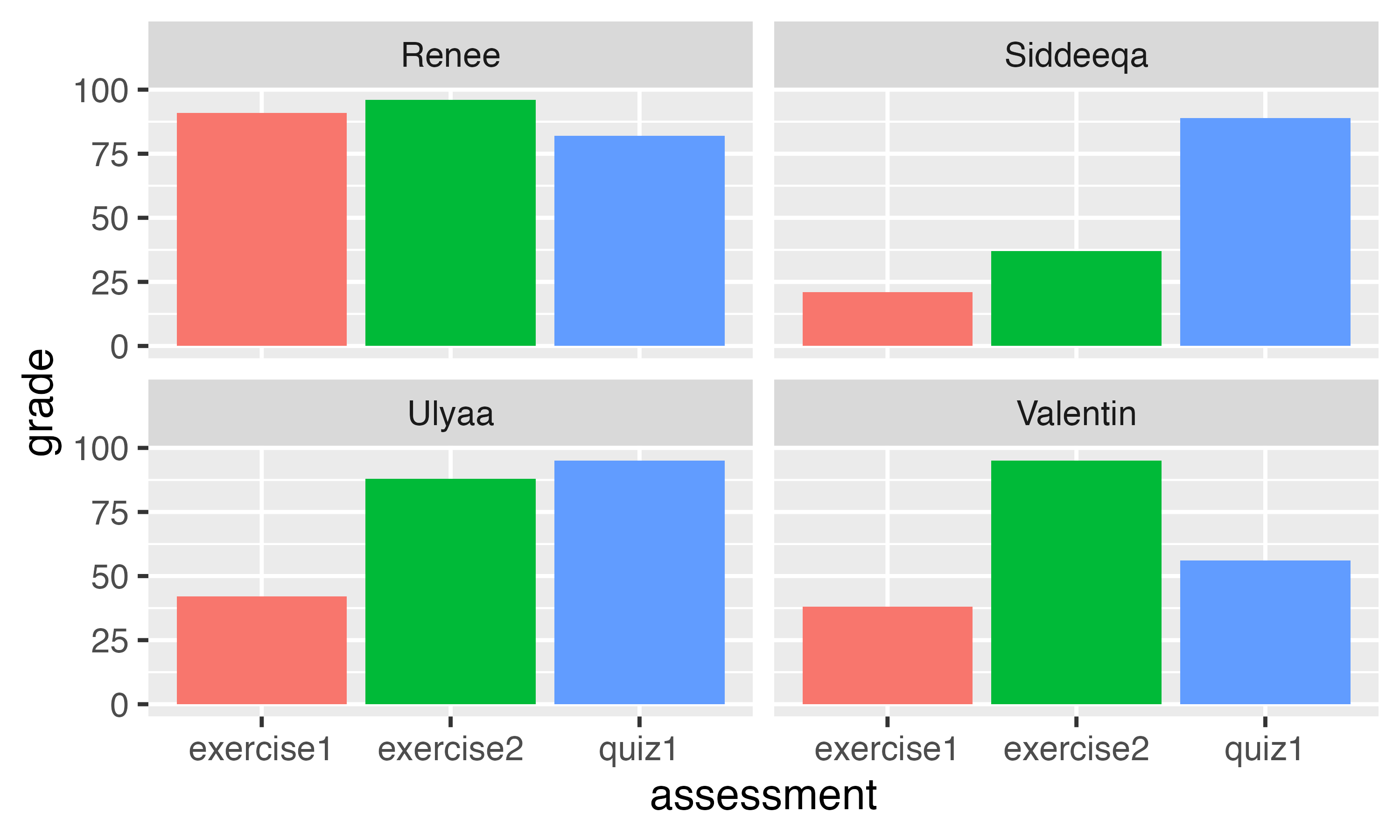
Common types of untidy data
- Column headers are values, not variable names
- Variables and values are not in rows or columns
- Multiple variables are stored in one column
Headers are values
| religion | <$10k | $10-20k | $20-30k | $30-40k | $40-50k | $50-75k |
|---|---|---|---|---|---|---|
| Agnostic | 27 | 34 | 60 | 81 | 76 | 137 |
| Atheist | 12 | 27 | 37 | 52 | 35 | 70 |
| Buddhist | 27 | 21 | 30 | 34 | 33 | 58 |
| Catholic | 418 | 617 | 732 | 670 | 638 | 1116 |
| Don’t know/refused | 15 | 14 | 15 | 11 | 10 | 35 |
| Evangelical Prot | 575 | 869 | 1064 | 982 | 881 | 1486 |
| Hindu | 1 | 9 | 7 | 9 | 11 | 34 |
| Historically Black Prot | 228 | 244 | 236 | 238 | 197 | 223 |
| Jehovah's Witness | 20 | 27 | 24 | 24 | 21 | 30 |
| Jewish | 19 | 19 | 25 | 25 | 30 | 95 |
| Mainline Prot | 289 | 495 | 619 | 655 | 651 | 1107 |
| Mormon | 29 | 40 | 48 | 51 | 56 | 112 |
| Muslim | 6 | 7 | 9 | 10 | 9 | 23 |
| Orthodox | 13 | 17 | 23 | 32 | 32 | 47 |
Headers are values
| religion | income | count |
|---|---|---|
| Agnostic | <$10k | 27 |
| Agnostic | $10-20k | 34 |
| Agnostic | $20-30k | 60 |
| Agnostic | $30-40k | 81 |
| Agnostic | $40-50k | 76 |
| Agnostic | $50-75k | 137 |
| Atheist | <$10k | 12 |
| Atheist | $10-20k | 27 |
| Atheist | $20-30k | 37 |
| Atheist | $30-40k | 52 |
| Atheist | $40-50k | 35 |
| Atheist | $50-75k | 70 |
| Buddhist | <$10k | 27 |
| Buddhist | $10-20k | 21 |
Variables not in table
| student | exercise1 | exercise2 | quiz1 |
|---|---|---|---|
| Ulyaa | 42 | 88 | 95 |
| Renee | 91 | 96 | 82 |
| Siddeeqa | 21 | 37 | 89 |
| Valentin | 38 | 95 | 56 |
| Key | |||
| Junior | |||
| Senior | |||
| Surprisingly high | |||
| Surprisingly low |
Variables not in table
| student | assessment | grade | class | surprise |
|---|---|---|---|---|
| Ulyaa | exercise1 | 42 | Junior | Low surprise |
| Ulyaa | exercise2 | 88 | Junior | |
| Ulyaa | quiz1 | 95 | Junior | High surprise |
| Renee | exercise1 | 91 | Senior | High surprise |
| Renee | exercise2 | 96 | Senior | High surprise |
| Renee | quiz1 | 82 | Senior | |
| Siddeeqa | exercise1 | 21 | Junior | Low surprise |
| Siddeeqa | exercise2 | 37 | Junior | Low surprise |
| Siddeeqa | quiz1 | 89 | Junior | |
| Valentin | exercise1 | 38 | Junior | Low surprise |
| Valentin | exercise2 | 95 | Junior | High surprise |
| Valentin | quiz1 | 56 | Junior |
Multiple variables in column
| iso2 | year | m014 | m1524 | m2534 | m3544 | f014 | f1524 | f2534 | f3544 |
|---|---|---|---|---|---|---|---|---|---|
| AD | 1996 | 0 | 0 | 0 | 4 | 0 | 1 | 1 | 0 |
| AD | 1997 | 0 | 0 | 1 | 2 | 0 | 1 | 2 | 3 |
| AD | 1998 | 0 | 0 | 0 | 1 | NA | NA | NA | NA |
| AD | 1999 | 0 | 0 | 0 | 1 | 0 | 0 | 0 | 1 |
| AD | 2000 | 0 | 0 | 1 | 0 | NA | NA | NA | NA |
| AD | 2001 | 0 | NA | NA | 2 | NA | NA | NA | NA |
| AD | 2002 | 0 | 0 | 0 | 1 | 0 | 1 | 0 | 0 |
| AD | 2003 | 0 | 0 | 0 | 1 | 0 | 1 | 1 | 1 |
| AD | 2004 | 0 | 0 | 0 | 1 | 0 | 0 | 1 | 0 |
| AD | 2005 | 0 | 0 | 1 | 1 | 0 | 1 | 1 | 1 |
| AD | 2006 | 0 | 1 | 1 | 2 | 0 | 0 | 1 | 0 |
| AD | 2007 | NA | NA | NA | NA | NA | NA | 1 | NA |
Multiple variables in column
| iso2 | year | sex | age | n |
|---|---|---|---|---|
| AD | 1996 | m | 014 | 0 |
| AD | 1996 | m | 1524 | 0 |
| AD | 1996 | m | 2534 | 0 |
| AD | 1996 | m | 3544 | 4 |
| AD | 1996 | f | 014 | 0 |
| AD | 1996 | f | 1524 | 1 |
| AD | 1996 | f | 2534 | 1 |
| AD | 1996 | f | 3544 | 0 |
| AD | 1997 | m | 014 | 0 |
| AD | 1997 | m | 1524 | 0 |
| AD | 1997 | m | 2534 | 1 |
| AD | 1997 | m | 3544 | 2 |
Your turn #2
| country | score_vault | score_floor |
|---|---|---|
| United States | 46.866 | 45.999 |
| Russia | 45.733 | 42.032 |
| China | 44.332 | 42.066 |
Your turn #2
| country | event | score |
|---|---|---|
| United States | vault | 46.866 |
| United States | floor | 45.999 |
| Russia | vault | 45.733 |
| Russia | floor | 42.032 |
| China | vault | 44.332 |
| China | floor | 42.066 |
Your turn #3
| country | 1957 | 1967 | 1977 | 1987 | 1997 | 2007 |
|---|---|---|---|---|---|---|
| Afghanistan | 30.332 | 34.020 | 38.438 | 40.822 | 41.763 | 43.828 |
| Albania | 59.280 | 66.220 | 68.930 | 72.000 | 72.950 | 76.423 |
| Algeria | 45.685 | 51.407 | 58.014 | 65.799 | 69.152 | 72.301 |
| Angola | 31.999 | 35.985 | 39.483 | 39.906 | 40.963 | 42.731 |
| Argentina | 64.399 | 65.634 | 68.481 | 70.774 | 73.275 | 75.320 |
| Australia | 70.330 | 71.100 | 73.490 | 76.320 | 78.830 | 81.235 |
| Austria | 67.480 | 70.140 | 72.170 | 74.940 | 77.510 | 79.829 |
| Bahrain | 53.832 | 59.923 | 65.593 | 70.750 | 73.925 | 75.635 |
Your turn #3
| country | year | lifeExp |
|---|---|---|
| Afghanistan | 1957 | 30.332 |
| Afghanistan | 1967 | 34.020 |
| Afghanistan | 1977 | 38.438 |
| Afghanistan | 1987 | 40.822 |
| Afghanistan | 1997 | 41.763 |
| Afghanistan | 2007 | 43.828 |
| Albania | 1957 | 59.280 |
| Albania | 1967 | 66.220 |
| Albania | 1977 | 68.930 |
Your turn #4
| country | vault_2012 | floor_2012 | vault_2016 | floor_2016 |
|---|---|---|---|---|
| United States | 48.132 | 45.366 | 46.866 | 45.999 |
| Russia | 46.366 | 41.599 | 45.733 | 42.032 |
| China | 44.266 | 40.833 | 44.332 | 42.066 |
Your turn #4
| country | event | year | score |
|---|---|---|---|
| United States | vault | 2012 | 48.132 |
| United States | floor | 2012 | 45.366 |
| United States | vault | 2016 | 46.866 |
| United States | floor | 2016 | 45.999 |
| Russia | vault | 2012 | 46.366 |
| Russia | floor | 2012 | 41.599 |
| Russia | vault | 2016 | 45.733 |
| Russia | floor | 2016 | 42.032 |
| China | vault | 2012 | 44.266 |
| China | floor | 2012 | 40.833 |
| China | vault | 2016 | 44.332 |
| China | floor | 2016 | 42.066 |
Pivoting
Pivoting longer
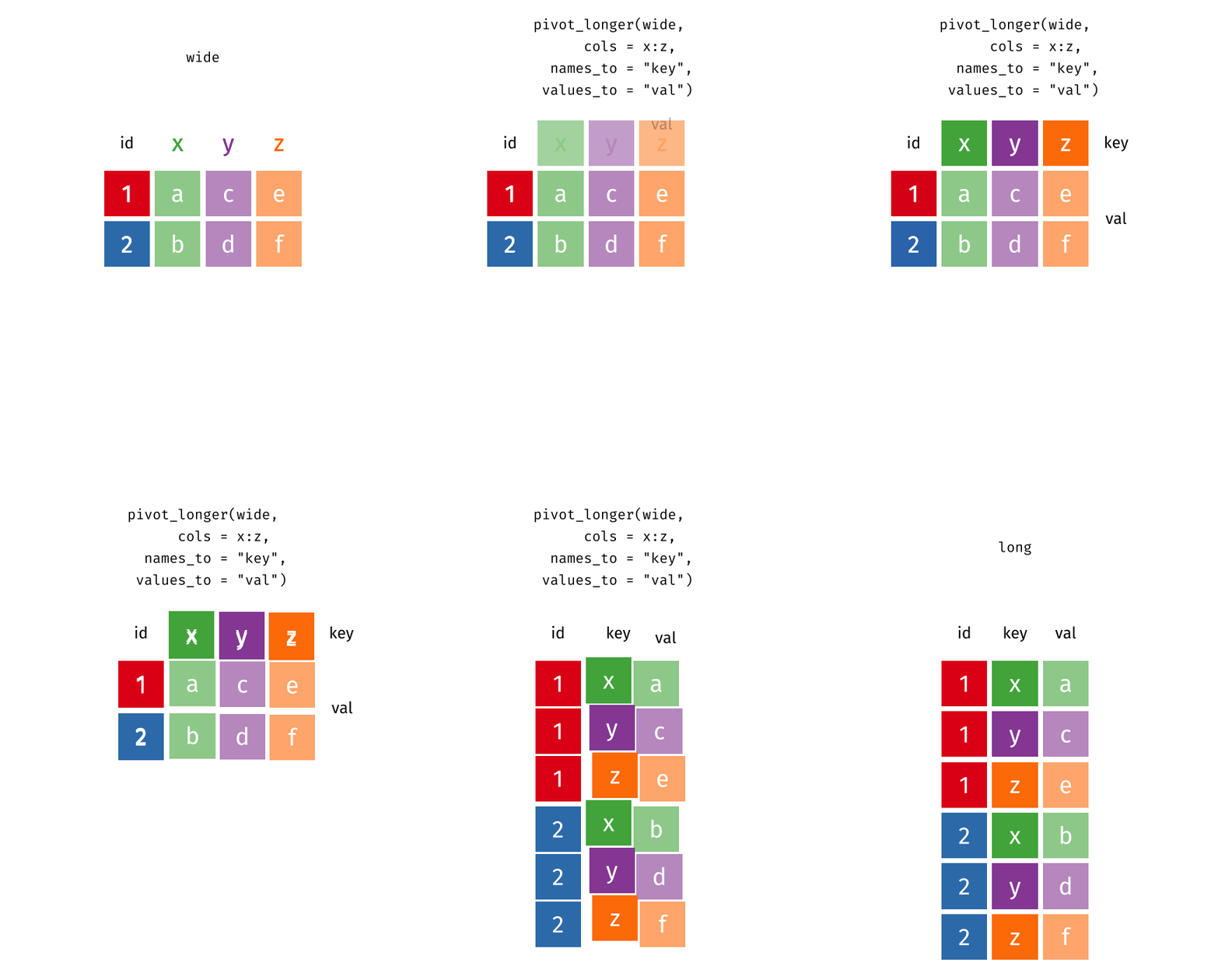
Pivoting longer
# A tibble: 12 × 3
   student  assessment grade
   <chr>    <chr>      <dbl>
 1 Ulyaa    exercise1     42
 2 Ulyaa    exercise2     88
 3 Ulyaa    quiz1         95
 4 Renee    exercise1     91
 5 Renee    exercise2     96
 6 Renee    quiz1         82
 7 Siddeeqa exercise1     21
 8 Siddeeqa exercise2     37
 9 Siddeeqa quiz1         89
10 Valentin exercise1     38
11 Valentin exercise2     95
12 Valentin quiz1 56Pivoting wider
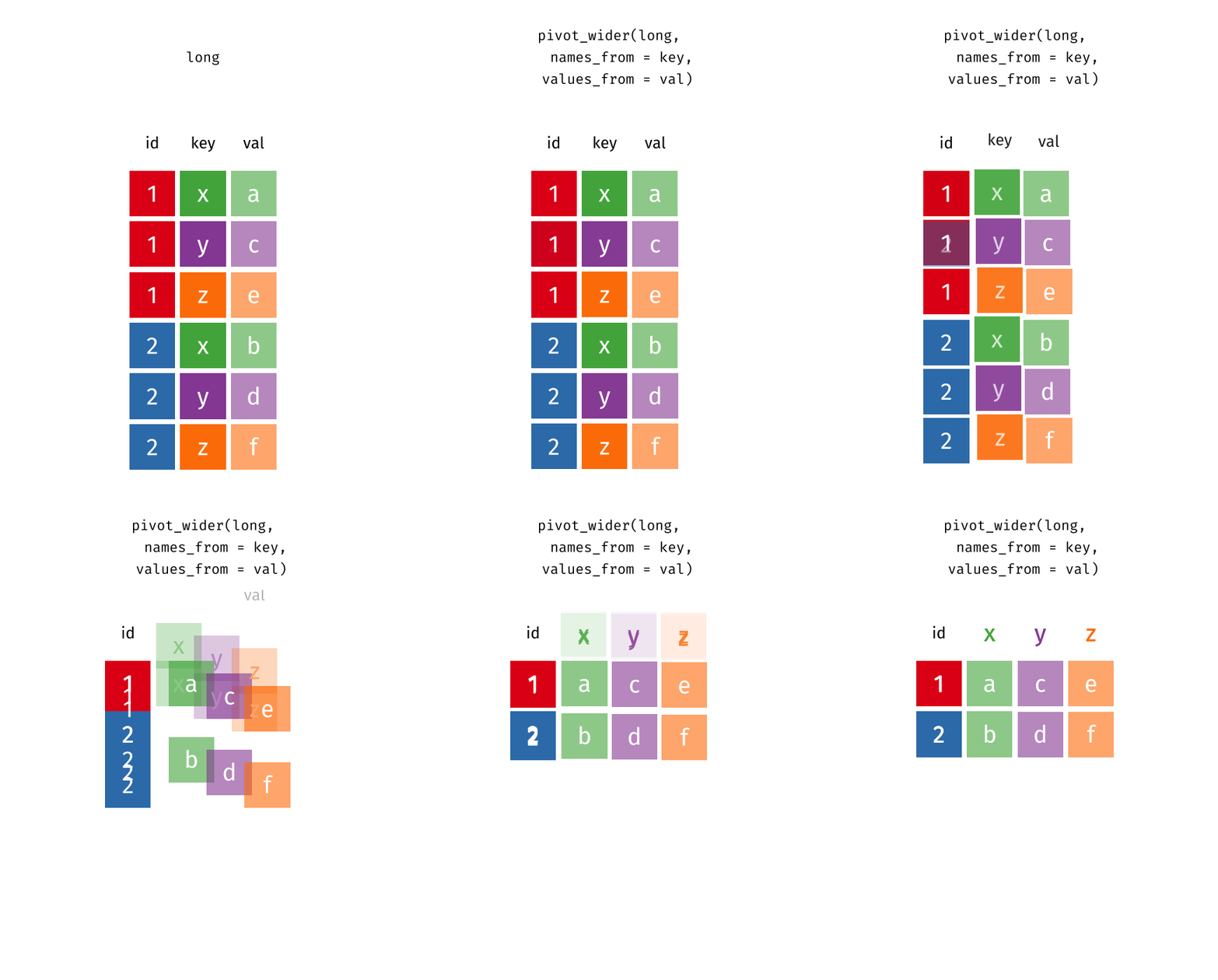
Pivoting wider
# A tibble: 12 × 3
   student  assessment grade
   <chr>    <chr>      <dbl>
 1 Ulyaa    exercise1     42
 2 Ulyaa    exercise2     88
 3 Ulyaa    quiz1         95
 4 Renee    exercise1     91
 5 Renee    exercise2     96
 6 Renee    quiz1         82
 7 Siddeeqa exercise1     21
 8 Siddeeqa exercise2     37
 9 Siddeeqa quiz1         89
10 Valentin exercise1     38
11 Valentin exercise2     95
12 Valentin quiz1 56Your/our turn #5
Pivoting!