Drawing lines with math
\[
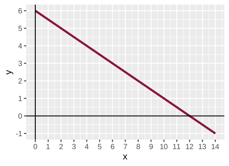
y = mx + b
\]
\(y\) A number
\(x\) A number
\(m\) Slope (\(\frac{\text{rise}}{\text{run}}\) )
\(b\) y-intercept
Draw some lines!
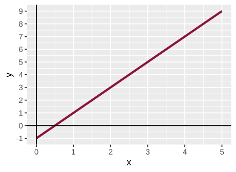
Sketch out the lines I give you in class!
Drawing lines with stats
\(y\) Outcome variable (Y )
\(\widehat{y}\)
\(x\) Explanatory variable (X )
\(x\)
\(m\) Slope
\(b_1\)
\(b\) y-intercept
\(b_0\)
The ^ hat on \(\widehat{y}\) is called a “hat”—we say “y hat”
It means it’s a fitted value , or the value on the line
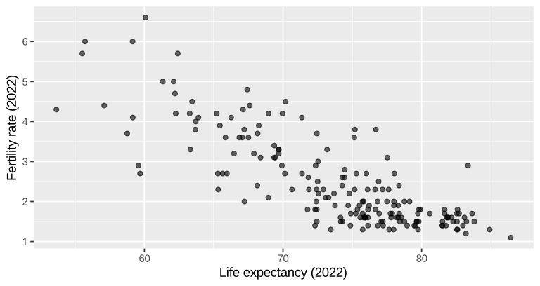
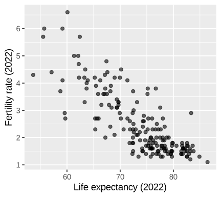
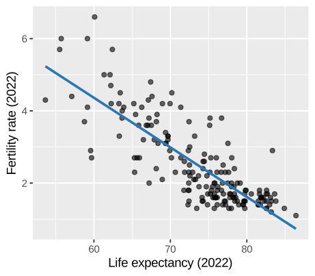
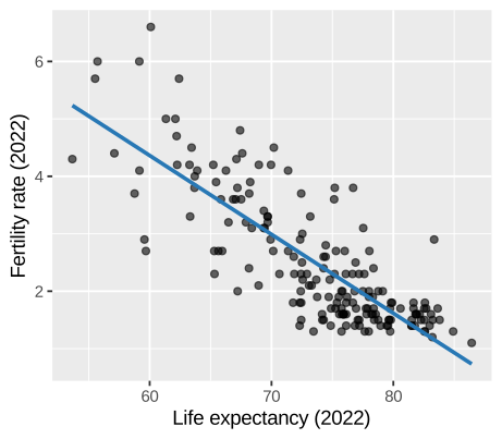
Fertility and life expectancy
\[
\widehat{y} = b_0 + b_1 x
\]
\[
\begin{aligned}
&\widehat{\text{fert}\_\text{rate}} = \\
&b_0 + b_1 \times \text{life}\_\text{exp}
\end{aligned}
\]
Building models in R
<- lm (< Y> ~ < X> , data = < DATA> )
lm() = l inear m odel<Y> ~ <X> is a model formula (same as in get_correlation()!)
library (moderndive)# Make the model <- lm (..., data = BLAH)# Coefficients in a nice table get_regression_table (name_of_model)# Fitted values and residuals for # every observation get_regression_points (name_of_model)
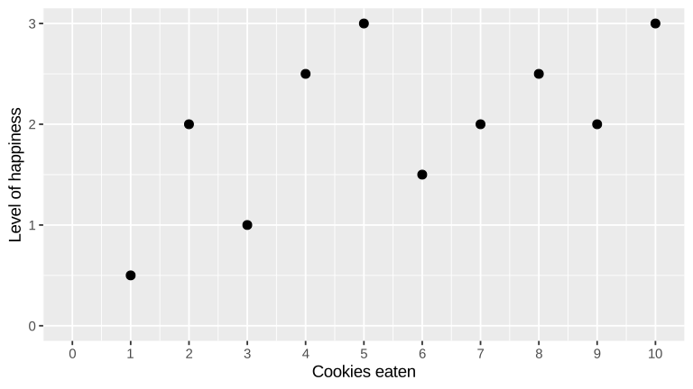
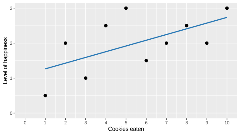
Cookies and happiness
\[
\begin{aligned}
&\widehat{\text{happiness}} = \\
&b_0 + b_1 \times \text{cookies}
\end{aligned}
\]
<- lm (~ cookies,data = cookies
Cookies and happiness
get_regression_table (cookies_model)
# A tibble: 2 × 7
  term      estimate std_error statistic p_value lower_ci upper_ci
  <chr>        <dbl>     <dbl>     <dbl>   <dbl>    <dbl>    <dbl>
1 intercept    1.1       0.47       2.34   0.047    0.016    2.18
2 cookies      0.164     0.076      2.16   0.063   -0.011    0.338
Translating results to math
term
estimate
intercept
1.100
cookies
0.164
\[
\begin{aligned}
&\widehat{\text{happiness}} = \\
&b_0 + b_1 \times \text{cookies}
\end{aligned}
\]
\[
\begin{aligned}
&\widehat{\text{happiness}} = \\
&1.1 + 0.164 \times \text{cookies}
\end{aligned}
\]
Template for the slope
A one unit increase in X is associated with a \(b_1\) increase (or decrease) in Y , on average
\[
\widehat{\text{happiness}} = 1.1 + 0.164 \times \text{cookies}
\]
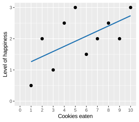
On average, eating one more cookie is associated with a 0.164 increase in happiness
Template for the intercept
\(b_0\) is the average value ofY when X is 0
\[
\widehat{\text{happiness}} = 1.1 + 0.164 \times \text{cookies}
\]
For someone who eats 0 cookies, the average level of happiness would be 1.1
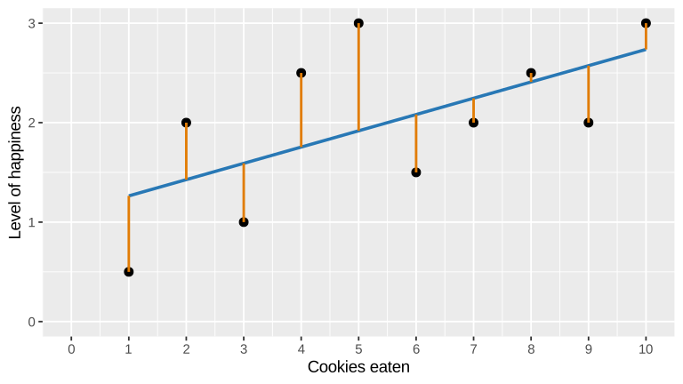
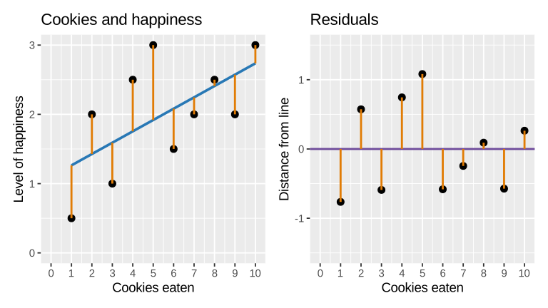
Observed vs. fitted values
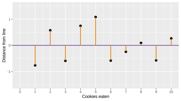
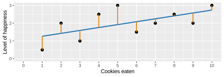
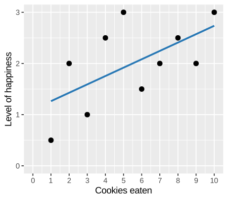
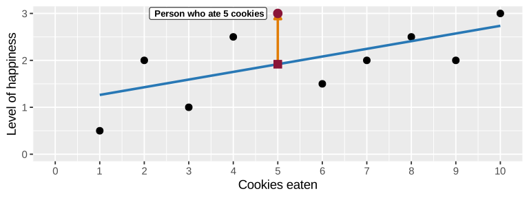
● Observed value (\(y\) ): Actual happiness = 3■ Fitted value (\(\widehat{y}\) ): \(1.1 + 0.164 \times 5 = 1.918\) ↓ Residual (\(y - \widehat{y}\) ): \(3 - 1.918 = 1.082\)
Residuals for every person
get_regression_points (cookies_model)
ID
happiness
cookies
happiness_hat
residual
1
0.5
1
1.264
-0.764
2
2.0
2
1.427
0.573
3
1.0
3
1.591
-0.591
4
2.5
4
1.755
0.745
5
3.0
5
1.918
1.082
6
1.5
6
2.082
-0.582
7
2.0
7
2.245
-0.245
8
2.5
8
2.409
0.091
9
2.0
9
2.573
-0.573
10
3.0
10
2.736
0.264
Fertility and life expectancy
\[
\begin{aligned}
&\widehat{\text{fert}\_\text{rate}} = \\
&b_0 + b_1 \times \text{life}\_\text{exp}
\end{aligned}
\]
<- lm (~ life_exp,data = UN_data_ch5
Fertility and life expectancy
get_regression_table (demographics_model)
# A tibble: 2 × 7
  term      estimate std_error statistic p_value lower_ci upper_ci
  <chr>        <dbl>     <dbl>     <dbl>   <dbl>    <dbl>    <dbl>
1 intercept   12.6       0.545      23.1       0   11.5     13.7
2 life_exp    -0.137     0.007     -18.6       0   -0.152   -0.123
(We’ll learn what all those other columns mean later in the semester!)
Translating results to math
term
estimate
intercept
12.599
life_exp
-0.137
\[
\begin{aligned}
&\widehat{\text{fert}\_\text{rate}} = \\
&b_0 + b_1 \times \text{life}\_\text{exp}
\end{aligned}
\]
\[
\begin{aligned}
&\widehat{\text{fert}\_\text{rate}} = \\
&12.6 + (-0.137) \times \text{life}\_\text{exp}
\end{aligned}
\]
Template for the slope
A one unit increase in X is associated with a \(b_1\) increase (or decrease) in Y , on average
\[
\widehat{\text{fert}\_\text{rate}} = 12.6 + (-0.137) \times \text{life}\_\text{exp}
\]
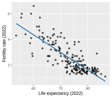
On average, a one-year increase in life expectancy is associated with a 0.137 decrease in the fertility rate
Use the right language!
“Associated”
Correlation isn’t causation! Adding a year of life to everyone in a country won’t make people have fewer kids. Wealthier, healthier, more educated countries tend to have both higher life expectancy and lower fertility
“On average”
Two countries with life expectancies one year apart won’t have fertility rates exactly 0.137 apart. Some are above the line, some below
Template for the intercept
\(b_0\) is the average value ofY when X is 0
\[
\widehat{\text{fert}\_\text{rate}} = 12.6 + (-0.137) \times \text{life}\_\text{exp}
\]
In a country where life expectancy is 0 years, the average fertility rate would be 12.6
A life expectancy of 0 is actually impossible, so this intercept has no practical meaning—it’s just where the line crosses the y-axis!
Correlation vs. slope
Correlation
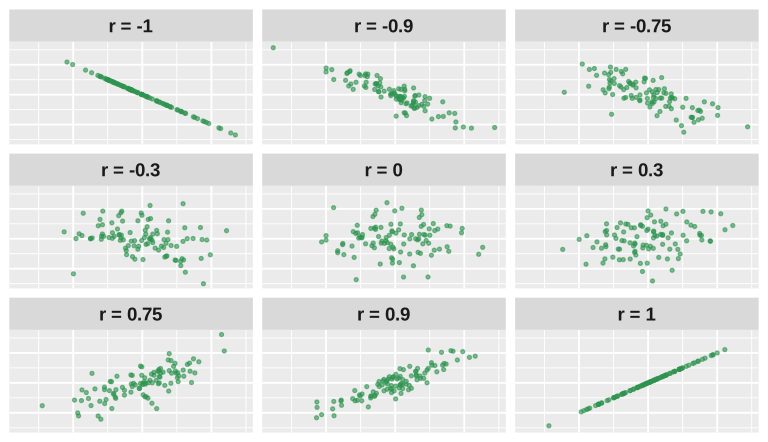
r = -0.812
Strength and direction of the relationship
Always between −1 and 1; no units
Slope
\(b_1\) = -0.137
Size of the relationship
Measured in units of Y per one unit of X
They’ll always have the same sign, but usually not the same value!
Observed vs. fitted values
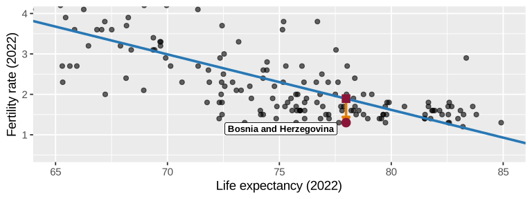
● Observed value (\(y\) ): Bosnia’s actual fertility rate = 1.3■ Fitted value (\(\widehat{y}\) ): \(12.599 + (-0.137) \times 77.98 = 1.894\) ↓ Residual (\(y - \widehat{y}\) ): \(1.3 - 1.894 = -0.594\)
Residuals for every country
get_regression_points (demographics_model)
iso
fert_rate
life_exp
fert_rate_hat
residual
AFG
4.3
53.65
5.234
-0.934
ALB
1.4
79.47
1.689
-0.289
DZA
2.7
78.03
1.887
0.813
AGO
5.0
62.11
4.072
0.928
ATG
1.6
77.80
1.918
-0.318
ARG
1.9
78.31
1.848
0.052
ARM
1.6
76.13
2.148
-0.548
AUS
1.6
83.09
1.192
0.408
Your turn #2
Does a country’s obesity rate predict its fertility rate?
Make a scatterplot of fert_rate and obes_rate
Find the correlation between the two with get_correlation()
Fit a model with lm() and look at the coefficients with get_regression_table()
Interpret the slope and the intercept