Multiple regression I

Quantitative Methods for
International Politics

IPOL 3270 • Fall 2026

October 4, 2026

Plan for today

Lines and regression (review)

Categories and regression

Multiple regression

Interpretation practice!

Lines and regression
(review)

Models

Models are simplified representations of complex things

Goal of regression

Use a model to explain (or predict) variation in an outcome using one or more explanatory variables

Drawing lines with stats

\(y = mx + b\) \(\widehat{y} = b_0 + b_1 x\)
\(y\) Outcome variable (Y) \(\widehat{y}\)
\(x\) Explanatory variable (X) \(x\)
\(m\) Slope \(b_1\)
\(b\) y-intercept \(b_0\)

Building models in R

name_of_model <- lm(<Y> ~ <X>, data = <DATA>)
  • lm() = linear model
  • <Y> ~ <X> is a model formula (same as in get_correlation()!)
library(moderndive)

# Make the model
name_of_model <- lm(..., data = BLAH)

# Coefficients in a nice table
get_regression_table(name_of_model)

# Fitted values and residuals for 
# every observation
get_regression_points(name_of_model)

cookies_model <- lm(
  happiness ~ cookies,
  data = cookies
)

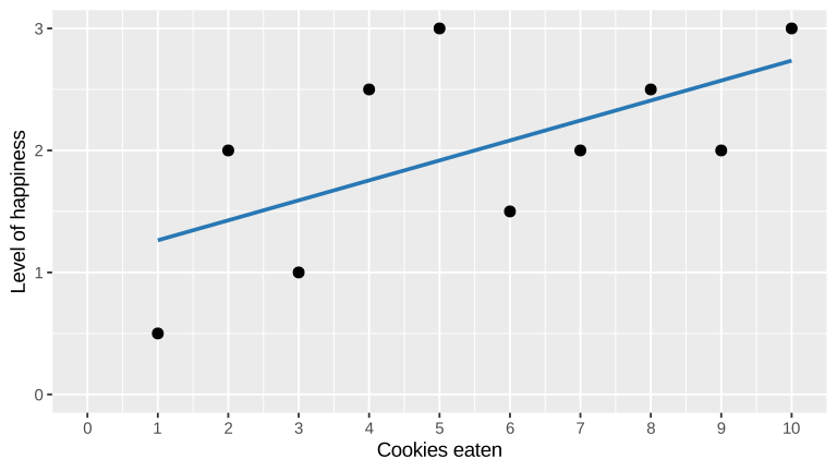
\[ \begin{aligned} \widehat{\text{happiness}} &= b_0 + b_1 \times \text{cookies} \\ \widehat{\text{happiness}} &= 1.1 + 0.164 \times \text{cookies} \end{aligned} \]

cookies_model |>
  get_regression_table() |>
  select(term, estimate)
# A tibble: 2 × 2
  term      estimate
  <chr>        <dbl>
1 intercept    1.1  
2 cookies      0.164

Templates (continuous X)

\[ \widehat{\text{happiness}} = b_0 + b_1 \times \text{cookies} \qquad \widehat{\text{happiness}} = 1.1 + 0.164 \times \text{cookies} \]

Parameter Term Template
Intercept \(b_0\) Average value of Y when X is 0
Slope \(b_1\) A one unit increase in X is associated with a \(b_1\) increase (or decrease) in Y, on average
Parameter Interpretation
Intercept Average happiness is 1.1 for someone who eats 0 cookies
Slope On average, eating one more cookie is associated with a 0.164 increase in happiness

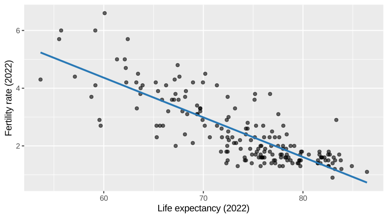
demographics_model <- lm(
  fert_rate ~ life_exp,
  data = UN_data_ch5
)

\[ \begin{aligned} \widehat{\text{fert}\_\text{rate}} &= b_0 + b_1 \times \text{life}\_\text{exp} \\ \widehat{\text{fert}\_\text{rate}} &= 12.61 + (-0.137) \times \text{life}\_\text{exp} \end{aligned} \]

demographics_model |>
  get_regression_table() |>
  select(term, estimate)
# A tibble: 2 × 2
  term      estimate
  <chr>        <dbl>
1 intercept   12.6  
2 life_exp    -0.137

Templates (continuous X)

\[ \widehat{\text{fert}\_\text{rate}} = b_0 + b_1 \times \text{life}\_\text{exp} \qquad \widehat{\text{fert}\_\text{rate}} = 12.61 + (-0.137) \times \text{life}\_\text{exp} \]

Parameter Term Template
Intercept \(b_0\) Average value of Y when X is 0
Slope \(b_1\) A one unit increase in X is associated with a \(b_1\) increase (or decrease) in Y, on average
Parameter Interpretation
Intercept In a country where life expectancy is 0 years, the average fertility rate would be 12.61
Slope On average, a one-year increase in life expectancy is associated with a 0.137 decrease in the fertility rate

Our turn #1

Does a country’s life expectancy predict its happiness?

Use simple-regression.qmd in the “Regression playground” project

  1. Make a scatterplot of happiness and life_expectancy
  2. Find the correlation between the two with get_correlation()
  3. Fit a model with lm() and look at the coefficients with get_regression_table()
  4. Interpret the slope and the intercept

Your turn #1

Does access to the internet predict national happiness?

  1. Make a scatterplot of happiness and internet_use_prop
  2. Find the correlation between the two with get_correlation()
  3. Fit a model with lm() and look at the coefficients with get_regression_table()
  4. Interpret the slope and the intercept

Categories
and regression

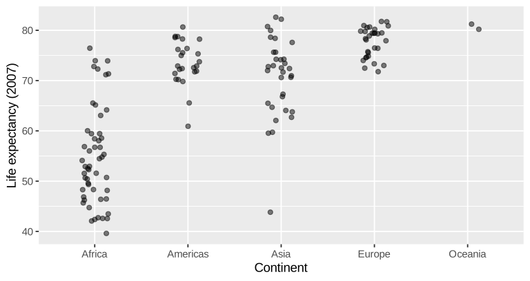
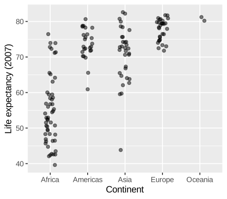
Life expectancy & continents (2007)

country continent lifeExp gdpPercap
Afghanistan Asia 43.828 975
Albania Europe 76.423 5,937
Algeria Africa 72.301 6,223
Angola Africa 42.731 4,797
Argentina Americas 75.320 12,779
Australia Oceania 81.235 34,435
Austria Europe 79.829 36,126
Bahrain Asia 75.635 29,796
Bangladesh Asia 64.062 1,391
Belgium Europe 79.441 33,693

Plot X and Y

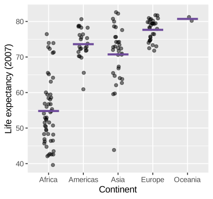
Averages for each continent

gapminder_2007 |>
  group_by(continent) |>
  summarize(
    n = n(),
    mean = mean(lifeExp),
    median = median(lifeExp)
  )
continent n mean median
Africa 52 54.81 52.93
Americas 25 73.61 72.9
Asia 33 70.73 72.4
Europe 30 77.65 78.61
Oceania 2 80.72 80.72

Can we draw a line through this?

  • X isn’t a number!
  • There’s no “one unit increase” in continent
  • …but lm() works anyway!

Building the model

lifeexp_model <- lm(lifeExp ~ continent, data = gapminder_2007)
get_regression_table(lifeexp_model)
# A tibble: 5 × 7
  term               estimate std_error statistic p_value lower_ci upper_ci
  <chr>                 <dbl>     <dbl>     <dbl>   <dbl>    <dbl>    <dbl>
1 intercept              54.8      1.02     53.4        0     52.8     56.8
2 continent-Americas     18.8      1.8      10.4        0     15.2     22.4
3 continent-Asia         15.9      1.65      9.68       0     12.7     19.2
4 continent-Europe       22.8      1.70     13.5        0     19.5     26.2
5 continent-Oceania      25.9      5.33      4.86       0     15.4     36.4

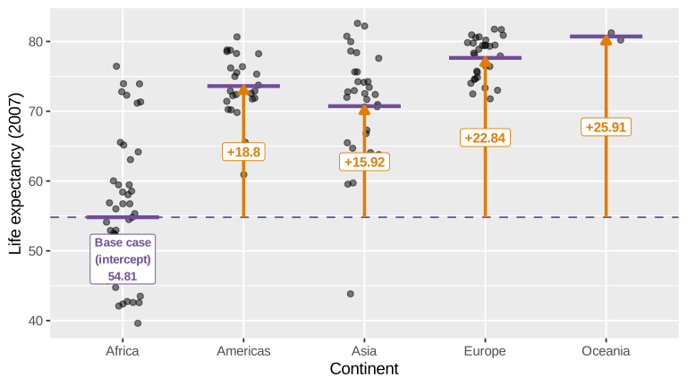
Where’d Africa go?!

The base case

One category gets left out and
becomes the base case

Also called the baseline, reference category, or omitted category

R uses the first category (alphabetically, by default) as the base case, so here it’s Africa

Every other coefficient is measured
relative to the base case

Translating results to math

term estimate
intercept 54.806
continent-Americas 18.802
continent-Asia 15.922
continent-Europe 22.843
continent-Oceania 25.913

\[ \begin{aligned} \widehat{\text{lifeExp}} = &\ b_0 + b_1 \times \text{Americas} + b_2 \times \text{Asia} \\ &+ b_3 \times \text{Europe} + b_4 \times \text{Oceania} \end{aligned} \]

\[ \begin{aligned} \widehat{\text{lifeExp}} = &\ 54.81 + 18.8 \times \text{Americas} + 15.92 \times \text{Asia} \\ &+ 22.84 \times \text{Europe} + 25.91 \times \text{Oceania} \end{aligned} \]

Switches

term estimate
intercept 54.806
continent-Americas 18.802
continent-Asia 15.922
continent-Europe 22.843
continent-Oceania 25.913

Template for the intercept

\(b_0\) is the average value of Y
for the base case

\[ \widehat{\text{lifeExp}} = 54.81 + 18.8 \times \text{Americas} + \dots \]

Average life expectancy in Africa is 54.81 years

All switches are off, so this is just the average of the base case

Template for the other coefficients

On average, Y is \(b\) higher (or lower) in this category, compared to the base case

\[ \widehat{\text{lifeExp}} = 54.81 + 18.8 \times \text{Americas} + \dots \]

On average, life expectancy in the Americas is 18.8 years higher than in Africa

It’s not “a one unit increase in continent”!
It’s the offset from the base case

Flip the switches!

Switch on \(\widehat{\text{lifeExp}}\)
None (Africa) \(54.81\)
Americas \(54.81 + 18.8 = 73.61\)
Asia \(54.81 + 15.92 = 70.73\)
Europe \(54.81 + 22.84 = 77.65\)
Oceania \(54.81 + 25.91 = 80.72\)
gapminder |> 
  filter(year == 2007) |> 
  group_by(continent) |> 
  summarise(avg = mean(lifeExp))
# A tibble: 5 × 2
  continent   avg
  <fct>     <dbl>
1 Africa     54.8
2 Americas   73.6
3 Asia       70.7
4 Europe     77.6
5 Oceania    80.7

These are just the averages for each continent!

Offsets from the base case

Observed vs. fitted values

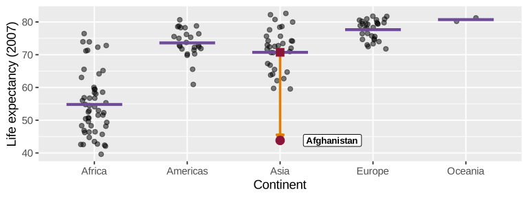
● Observed value (\(y\)): Afghanistan’s actual life expectancy = 43.83
■ Fitted value (\(\widehat{y}\)): \(54.81 + 15.92 \times 1 = 70.73\) (the Asia average)
↓ Residual (\(y - \widehat{y}\)): \(43.83 - 70.73 = -26.9\)

Residuals for every country

get_regression_points(lifeexp_model, ID = "country")
country lifeExp continent lifeExp_hat residual
Afghanistan 43.828 Asia 70.728 -26.900
Albania 76.423 Europe 77.649 -1.226
Algeria 72.301 Africa 54.806 17.495
Angola 42.731 Africa 54.806 -12.075
Argentina 75.320 Americas 73.608 1.712
Australia 81.235 Oceania 80.720 0.516
Austria 79.829 Europe 77.649 2.180
Bahrain 75.635 Asia 70.728 4.907

Templates (categorical X)

\[ \begin{aligned} \widehat{\text{lifeExp}} = &\ 54.81 + 18.8 \times \text{Americas} + 15.92 \times \text{Asia} \\ &+ 22.84 \times \text{Europe} + 25.91 \times \text{Oceania} \end{aligned} \]

Parameter Term Template
Intercept \(b_0\) Average value of Y for the base case
Coefficient \(b_n\) On average, Y is \(b_n\) higher (or lower) in this category, compared to the base case
Parameter Interpretation
Intercept Average life expectancy in Africa is 54.81 years
Americas On average, life expectancy in the Americas is 18.8 years higher than in Africa

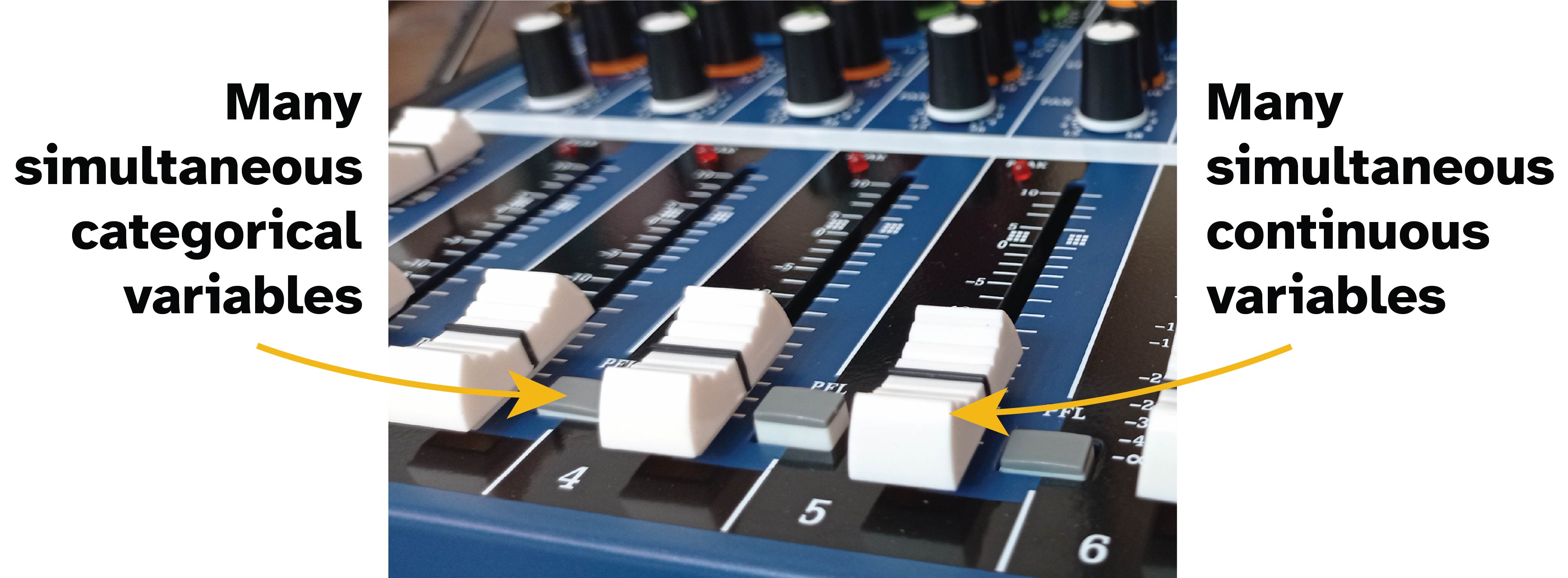
Sliders and switches

Categorical X

Y shifts by \(b_n\)
compared to the base case

Continuous X

Y changes by \(b_n\)

Our turn #2

Is happiness different across continents?

Keep using simple-regression.qmd

  1. Make a plot of happiness across continent
  2. Find the average happiness in each continent with group_by() and summarize()
  3. Fit a model with lm() and look at the coefficients with get_regression_table()
  4. Interpret the intercept and the coefficient for Europe

Your turn #2

Is internet access different across continents?

Keep using simple-regression.qmd

  1. Make a plot of internet_use_prop across continent
  2. Find the average internet_use_prop in each continent with group_by() and summarize()
  3. Fit a model with lm() and look at the coefficients with get_regression_table()
  4. Interpret the intercept and the coefficient for Asia

Multiple regression

Many explanations!

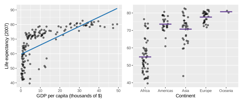
Wealth and continent-level differences each explain some of the variation in life expectancy

One at a time

gdp_model <- lm(
  lifeExp ~ gdp_1000,
  data = gapminder_2007
)

gdp_model |>
  get_regression_table() |>
  select(term, estimate)
# A tibble: 2 × 2
  term      estimate
  <chr>        <dbl>
1 intercept   59.6  
2 gdp_1000     0.637
lifeexp_model <- lm(
  lifeExp ~ continent,
  data = gapminder_2007
)

lifeexp_model |>
  get_regression_table() |>
  select(term, estimate)
# A tibble: 5 × 2
  term               estimate
  <chr>                 <dbl>
1 intercept              54.8
2 continent-Americas     18.8
3 continent-Asia         15.9
4 continent-Europe       22.8
5 continent-Oceania      25.9

Both at the same time

GDP per capita and continent both explain
some variation in life expectancy

  • On its own, a $1,000 increase in GDP per capita is associated with a 0.64 year increase in life expectancy, on average
  • On its own, life expectancy in Europe is 22.84 years higher than in Africa, on average

Some of that explanation is shared!

Richer countries are concentrated in some continents, so each variable is partly getting credit for the other

Building the model

Add more explanatory variables with +

lifeexp_lots_model <- lm(lifeExp ~ gdp_1000 + continent, data = gapminder_2007)
get_regression_table(lifeexp_lots_model)
# A tibble: 6 × 7
  term               estimate std_error statistic p_value lower_ci upper_ci
  <chr>                 <dbl>     <dbl>     <dbl>   <dbl>    <dbl>    <dbl>
1 intercept            53.7       0.928     57.9    0       51.9     55.6  
2 gdp_1000              0.347     0.057      6.11   0        0.234    0.459
3 continent-Americas   16.1       1.66       9.66   0       12.8     19.3  
4 continent-Asia       12.7       1.56       8.14   0        9.59    15.7  
5 continent-Europe     15.2       1.96       7.79   0       11.4     19.1  
6 continent-Oceania    16.6       4.97       3.35   0.001    6.81    26.5  

Translating results to math

term estimate
intercept 53.735
gdp_1000 0.347
continent-Americas 16.059
continent-Asia 12.669
continent-Europe 15.228
continent-Oceania 16.650

\[ \begin{aligned} \widehat{\text{lifeExp}} = &\ b_0 + b_1 \times \text{GDP}_{1000} + b_2 \times \text{Americas} + b_3 \times \text{Asia} \\ &+ b_4 \times \text{Europe} + b_5 \times \text{Oceania} \end{aligned} \]

\[ \begin{aligned} \widehat{\text{lifeExp}} = &\ 53.74 + 0.347 \times \text{GDP}_{1000} + 16.06 \times \text{Americas} + 12.67 \times \text{Asia} \\ &+ 15.23 \times \text{Europe} + 16.65 \times \text{Oceania} \end{aligned} \]

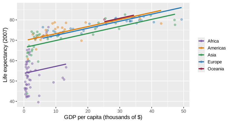
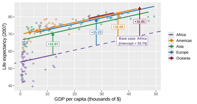
One line per continent

Same slope for GDP (0.347) in every continent; the continent switches shift the intercept

Switches shift the line

Each continent’s coefficient is how far its line is shifted above (or below) Africa’s line

Filtering out variation

Each X in the model explains
some portion of the variation in Y

This will often change the simple regression coefficients

On its own In the model with both
GDP per capita ($1,000s) 0.637 0.347
Europe 22.84 15.23

Interpretation is trickier, since you can only ever move one slider or switch at a time

Templates (multiple X)

\[ \widehat{y} = b_0 + b_1 \times x_1 + b_2 \times x_2 + \dots + b_n \times x_n \]

\[ \begin{aligned} \widehat{\text{lifeExp}} = &\ b_0 + b_1 \times \text{GDP}_{1000} + b_2 \times \text{Americas} + b_3 \times \text{Asia} \\ &+ b_4 \times \text{Europe} + b_5 \times \text{Oceania} \end{aligned} \]

Parameter Term Template
Intercept \(b_0\) Average value of Y when all continuous Xs are 0 and all categorical Xs are the base case
Continuous \(b_n\) Taking all other variables in the model into account, a one unit increase in Xn is associated with a \(b_n\) increase (or decrease) in Y, on average
Categorical \(b_n\) Taking all other variables in the model into account, Y is \(b_n\) higher (or lower) in this category compared to the base case, on average

Templates (multiple X)

\[ \begin{aligned} \widehat{\text{lifeExp}} = &\ 53.74 + 0.347 \times \text{GDP}_{1000} + 16.06 \times \text{Americas} + 12.67 \times \text{Asia} \\ &+ 15.23 \times \text{Europe} + 16.65 \times \text{Oceania} \end{aligned} \]

Parameter Interpretation
Intercept In an African country with a GDP per capita of $0, average life expectancy would be 53.74 years
GDP Controlling for continent, a $1,000 increase in GDP per capita is associated with a 0.35 year increase in life expectancy, on average
Europe Controlling for GDP per capita, life expectancy in Europe is 15.23 years higher than in Africa, on average

“Controlling for…”

  • Controlling for…
  • Taking all other variables in the model into account…
  • Holding … constant
  • Accounting for…
  • Adjusting for…

These all mean the same thing—we’re comparing countries that have the same values for every other variable in the model, or filtering out the variation that comes from the other variables and isolating just one slider or switch

Lots of sliders and switches!

un_model <- lm(
  life_exp ~ fert_rate +
    gdp_1000 + continent,
  data = un_data
)
  • Sliders: fertility rate and GDP per capita
  • Switches: continent (Africa is the base case)
un_model |> 
  get_regression_table() |> 
  select(term, estimate)
# A tibble: 8 × 2
  term                    estimate
  <chr>                      <dbl>
1 intercept                 79.3  
2 fert_rate                 -3.48 
3 gdp_1000                   0.092
4 continent-Asia             1.88 
5 continent-Europe           2.10 
6 continent-North America    1.78 
7 continent-Oceania          4.57 
8 continent-South America    1.87 

Move one slider/switch at a time

Imagine an African country with a fertility rate of 3 and a GDP per capita of $10,000

Scenario Fertility rate GDP per capita Continent Predicted life exp. Change
Start 3 $10,000 Africa 69.78 0.000
Fertility + 1 4 $10,000 Africa 66.29 -3.482
GDP + $1,000 3 $11,000 Africa 69.87 0.092
Europe 3 $10,000 Europe 71.87 2.097

You can only interpret one slider or switch at a time;
keep the others constant

Interpreting everything

Parameter Interpretation
Intercept In an African country with a fertility rate of 0 and a GDP per capita of $0, average life expectancy would be 79.3 years (not a real country!)
Fertility Taking GDP per capita and continent into account, a one-child increase in the fertility rate is associated with a 3.48 year decrease in life expectancy, on average
GDP Holding fertility and continent constant, a $1,000 increase in GDP per capita is associated with a 0.092 year increase in life expectancy, on average
Europe Controlling for fertility and GDP per capita, life expectancy in Europe is 2.1 years higher than in Africa, on average

Our turn #3

Is national happiness explained by wealth, internet access, and continent?

Use multiple-regression.qmd in the “Regression playground” project

  1. Fit a model with lm() that explains happiness with gdp_per_cap_1000, internet_use_prop, and continent
  2. Look at the coefficients with get_regression_table()
  3. Write out the model as an equation
  4. Interpret the intercept and the coefficients for GDP per capita, internet use, and Europe

Your turn #3

Is national happiness explained by health, jobs, and income?

  1. Fit a model that explains happiness with life_expectancy, unemployment_rate, and income_group
  2. Look at the coefficients with get_regression_table()
  3. What’s the base case for income_group?
  4. Interpret the coefficients for life expectancy, unemployment, and high income

Interpretation
practice!

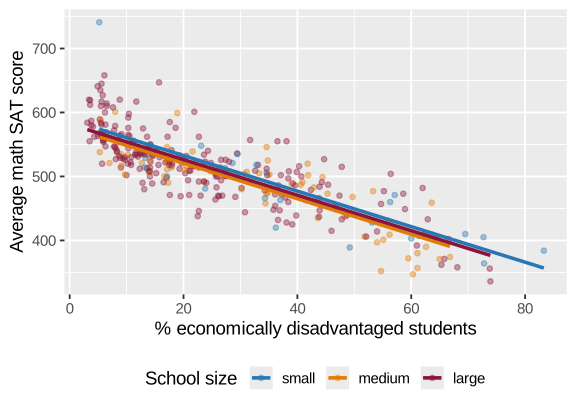
SAT scores in Massachusetts

\[ \begin{aligned} \widehat{\text{SAT}\_\text{math}} =&\ 588.19 + (-2.78) \times \text{perc}\_\text{disadvan}\ + \\ & (-11.91) \times \text{medium} + (-6.36) \times \text{large} \end{aligned} \]

lm(average_sat_math ~
     perc_disadvan + size,
   data = MA_schools)
term estimate
intercept 588.190
perc_disadvan -2.777
size-medium -11.913
size-large -6.362

SAT scores in Massachusetts

  • Intercept: A small school with 0% economically disadvantaged students would have an average math SAT score of 588.19
  • % disadvantaged: Controlling for school size, a one percentage point increase in economically disadvantaged students is associated with a 2.78 point decrease in average math SAT scores, on average
  • Medium: Taking the % of disadvantaged students into account, medium schools score 11.91 points lower than small schools, on average
  • Large: Taking the % of disadvantaged students into account, large schools score 6.36 points lower than small schools, on average

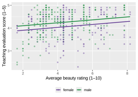
Teaching evaluations

\[ \widehat{\text{score}} = 4.06 + (-0.006) \times \text{age} + 0.064 \times \text{bty}\_\text{avg} + 0.201 \times \text{male} \]

lm(score ~ age + bty_avg + gender,
   data = evals)
term estimate
intercept 4.055
age -0.006
bty_avg 0.064
gender-male 0.201

Teaching evaluations

  • Intercept: A 0-year-old female professor with a beauty rating of 0 would have an average evaluation score of 4.06 (not a real professor!)
  • Age: Controlling for beauty and gender, a one-year increase in a professor’s age is associated with a 0.006 point decrease in evaluation scores, on average
  • Beauty: Holding age and gender constant, a one-point increase in beauty rating is associated with a 0.064 point increase in evaluation scores, on average
  • Male: Taking age and beauty into account, male professors have evaluation scores that are 0.201 points higher than female professors, on average

Penguin weights

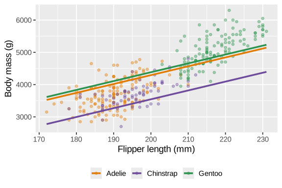
\[ \begin{aligned} \widehat{\text{body}\_\text{mass}} = &\ (-3904.4) + 27.4 \times \text{flipper}\_\text{len} + 61.7 \times \text{bill}\_\text{len} \\ &+ (-748.6) \times \text{Chinstrap} + 90.4 \times \text{Gentoo} \end{aligned} \]

lm(body_mass ~ flipper_len +
     bill_len + species,
   data = penguins)
term estimate
intercept -3904.387
flipper_len 27.429
bill_len 61.736
species-Chinstrap -748.562
species-Gentoo 90.435

Penguin weights

  • Intercept: An Adelie penguin with 0 mm flippers and a 0 mm bill would weigh -3904.4 grams (not a real penguin!)
  • Flipper length: Controlling for bill length and species, a one-mm increase in flipper length is associated with a 27.4 gram increase in body mass, on average
  • Bill length: Holding flipper length and species constant, a one-mm increase in bill length is associated with a 61.7 gram increase in body mass, on average
  • Chinstrap: Taking flipper and bill length into account, Chinstrap penguins weigh 748.6 grams less than Adelie penguins, on average
  • Gentoo: Taking flipper and bill length into account, Gentoo penguins weigh 90.4 grams more than Adelie penguins, on average

House prices

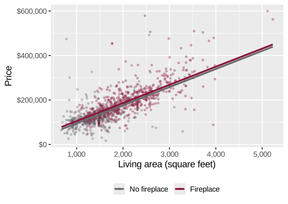
\[ \widehat{\text{price}} = 20{,}366 + 81.47 \times \text{living}\_\text{area} + (-242.86) \times \text{age} + 10{,}293 \times \text{fireplace} \]

lm(price ~ living_area +
     age + fireplace,
   data = saratoga_houses)
term estimate
intercept 20365.805
living_area 81.469
age -242.860
fireplaceTRUE 10292.582

House prices

  • Intercept: A brand new house with 0 square feet and no fireplace would cost $20,366 (not a real house!)
  • Living area: Controlling for age and fireplaces, a one-square-foot increase in living area is associated with a $81.47 increase in price, on average
  • Age: Holding living area and fireplaces constant, a one-year increase in a house’s age is associated with a $242.86 decrease in price, on average
  • Fireplace: Taking living area and age into account, houses with a fireplace cost $10,293 more than houses without one, on average