Sampling I & II

Quantitative Methods for
International Politics

IPOL 3270 • Fall 2026

October 25, 2026

Plan for today

Populations and samples

M&Ms

Sampling variation

Uncertainty

Choosing a sample size

Populations
and samples

Data so far

World happiness, Gapminder, V-Dem, UN data
(Nearly) every country
Regression coefficients describe entire countries
We can (theoretically) measure every country

But often we can’t measure everything we care about

The Arab Barometer

Huge public opinion survey in the Middle East and North Africa
Wave 8 (2023–2024): 15,627 people in 8 countries
Face-to-face interviews in random households

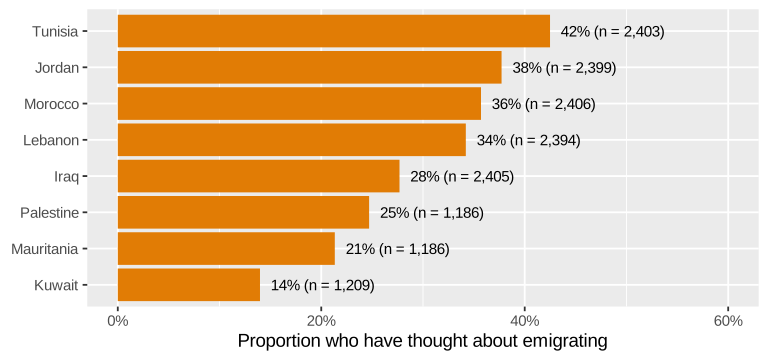
Some people decide to leave their countries to live somewhere else. Have you ever thought about emigrating from [your country]?

Thought about emigrating?

42% of all Tunisians? From only 2,403 people?

Population vocabulary

Population

A collection of things in the world

People, countries, voters, MPs, exports, aid projects, legislation

All adults in Tunisia

Population parameter

Something we want to know about the population

Average life expectancy in GCC countries
Median commute time in Doha
Relationship between poverty and fertility rates

Proportion of all Tunisian adults who have thought about emigrating (p)

Parameters are what you measure to answer research questions

Also called “estimands”—the thing you care about

Counting the population

Census

Measure every single thing
in the population

Expensive, slow, often impossible

Sampling

Only measure a part of the population

Interview 2,403 Tunisians

Measuring the sample

Sample statistic
(or point estimate)

The population parameter (or estimand), but calculated from a sample of the population

Uses a hat! \widehat{p} = 0.425

Same hat as \widehat{y} in regression: hat = estimate

Parameters and statistics

	Population parameter	Sample statistic
Proportion	p	\widehat{p}
Mean	\mu	\bar{x}
Regression slope	\beta_1	b_1 or \widehat{\beta}_1

Everything you calculate from a sample is an estimate of some unknown population value

Is the sample any good?

Representative: Does the sample look like the population?
Unbiased: Did every part of the population have the same chance of being picked?
Generalizable: Is \widehat{p} a good guess for p?

Random sampling fixes all these

What if we want to save money
and we just run an online survey?

33% of Tunisians don’t use the internet
They’re much less likely to have thought about emigrating
An online survey only sees internet users: 51% instead of 42%

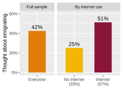
Even if we surveyed a million Tunisians online,
our parameter would be wrong!

M&Ms

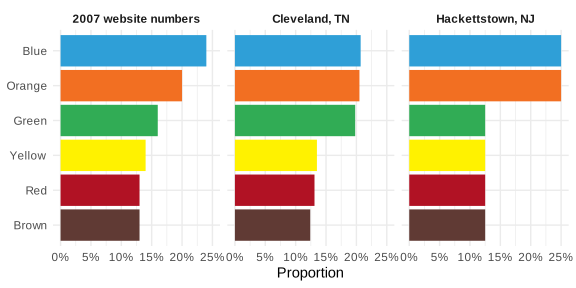
M&M colors!

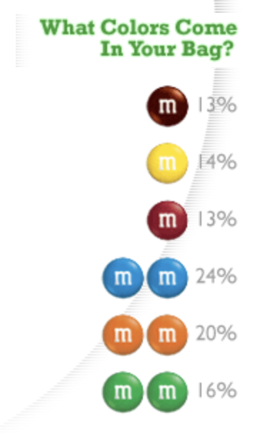
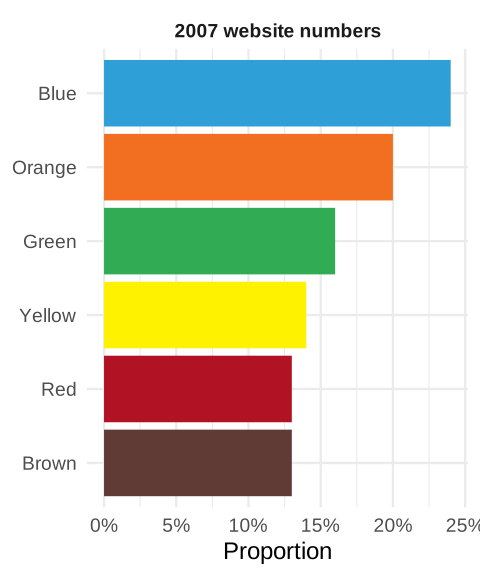
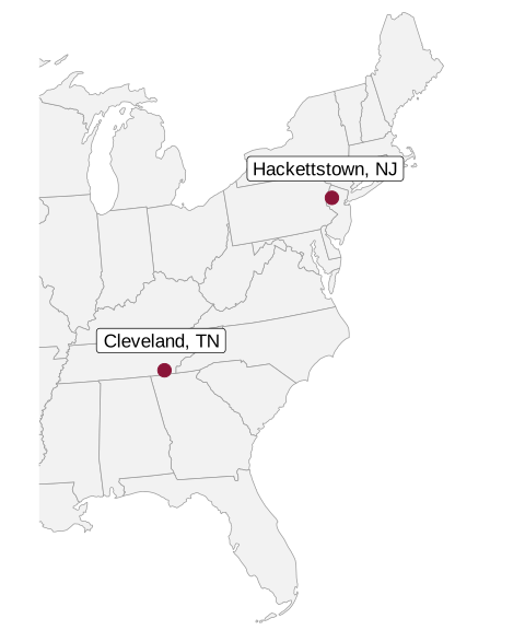
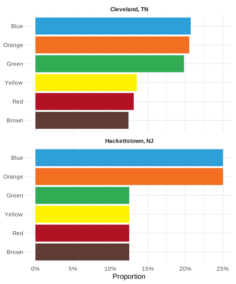
What about Qatar?

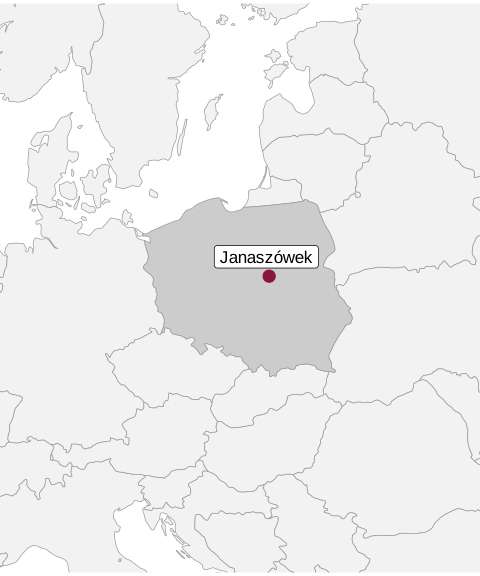
Mars Polska

Your bag is a sample

Every bag was filled from a giant vat (kind of) of M&Ms at the Mars factory in Janaszówek, Poland
Each bag has ≈50 M&Ms
We want to know what the factory makes, but we only have our bags

Define the population

Population

Every plain M&M made in Janaszówek

Population parameter

The proportion of each color in the vat

p_\text{blue}, p_\text{brown}, p_\text{green},
p_\text{orange}, p_\text{red}, p_\text{yellow}

Census or sample?

Census

Count every single M&M made in Poland (ever? on a specific day?)

Impossible!

Sample

Count the M&Ms in one bag

\widehat{p}_\text{green} = green M&Ms in your bag ÷ all M&Ms in your bag

Your turn: count your bag

Don’t eat anything yet!
Count how many M&Ms of each color are in your bag
Calculate \widehat{p} for each color (count ÷ total)
Fill out the form here:

andhs.co/mms

Color	Count	\widehat{p}
Blue
Brown
Green
Orange
Red
Yellow
Total		1.00

Is your bag a good sample?

Representative: Does your bag look like the vat?
Unbiased: Did every M&M have the same chance of ending up in your bag?
Generalizable: Is your \widehat{p}_\text{green} a good guess for p_\text{green}?

What could go wrong?

All our bags came from the same two boxes at Carrefour
Are our bags a random sample of all bags?

Who’s right?

Compare your \widehat{p}_\text{green} with your neighbors
Everyone’s bag gives a different answer
Nobody did anything wrong!

Every sample is a little different:
sampling variation

Getting a better estimate

More bags?
Bigger bags?
Pool the whole class into one giant sample!

Bigger samples → better estimates

Our class’s estimate

Let’s look at the data!

Everyone’s \widehat{p}_\text{green}: how spread out are they?
Pool all our bags into one giant sample
Compare our pooled \widehat{p}_\text{green} with Cleveland (19.8%), Hackettstown (12.5%), and the 2007 numbers (16%)

What did we find?

Whose bag was closest to the pooled estimate? Farthest?
How different were the individual bags from each other?
Is our pooled estimate closer to one of the US factories?
Do you trust the pooled estimate more than your own bag? Why?

Plan for today

Sampling variation

Uncertainty

Choosing a sample size

Sampling variation

What our bags taught us

Every bag gave a different \widehat{p}_\text{green}
One small bag can be way off
Pooling all our bags into one big sample gave a much better estimate
A few big samples beat lots of little ones

Today: why that works and how much better bigger samples are

We can’t buy 1,000 bags

Our class’s bags give us a rough picture of sampling variation
To really see it, we’d need thousands of bags
And we still wouldn’t know the true p_\text{green}!

Computers to the rescue!

Simulation

Make a pretend population where we know the truth, then take lots of random samples from it

Build a population with a known parameter
Draw a random sample
Calculate the statistic (\widehat{p})
Repeat thousands of times
Look at all the \widehat{p}s

A virtual vat

10,000 simulated M&Ms (using our class’s pooled colors)
True p_\text{green} = 0.173
Each virtual bag = 50 random M&Ms from the vat

mm_vat |>
  rep_slice_sample(
    n = 50, reps = 1000
  ) |>
  summarize(
    p_hat = mean(color == "green")
  )

1,000 virtual bags

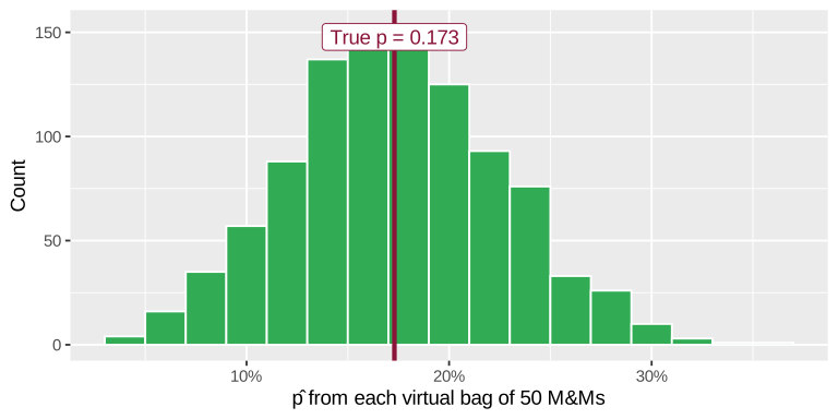
Centered on the truth, but lots of bags are way off—just like our real bags!

Same idea, but with real survey data

Pretend the 2,403 Tunisian respondents are the entire population

We know the true parameter: p = 0.425

What happens if we take random samples of 100 people from this population?

Sample	Yes	\widehat{p}
1	40	0.4
2	40	0.4
3	43	0.43
4	44	0.44
5	39	0.39

Every sample gives a different \widehat{p}
None of them are exactly 0.425
That’s fine! It’s just sampling variation

Repeat 1,000 times

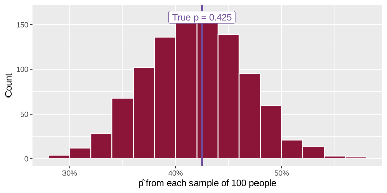
This is a sampling distribution

Sampling distribution

The distribution of a statistic (like \widehat{p}) across lots of random samples of the same size

Shows how much estimates bounce around from sample to sample
We can only see it with simulation (or math)
In real life, you only get one draw from it!

Three different distributions

Population

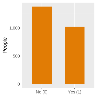
All 2,403 Tunisians’ answers

One sample

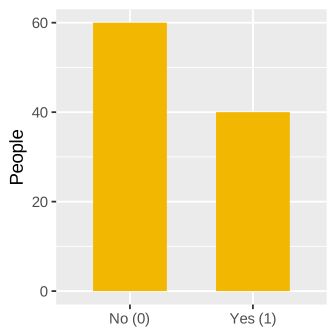
100 people’s answers
(\widehat{p} = 0.4)

Sampling distribution

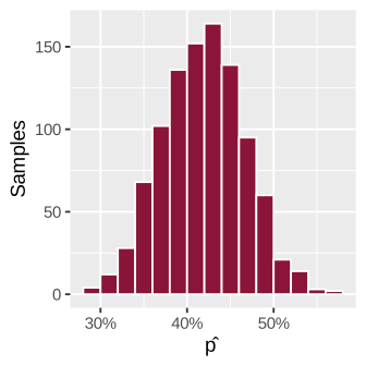
1,000 samples’ \widehat{p}s

Statistics have distributions too!

More samples or bigger samples?

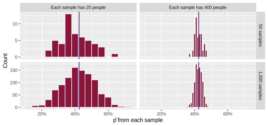
More samples → smoother picture of the same distribution; bigger samples → narrower distribution

Central limit theorem

With random samples, the sampling distribution of a sample proportion (or mean) is approximately normal

…centered at the population parameter (p)
…no matter what the population looks like (ours was just 0s and 1s!)
…as long as the samples are big enough

\widehat{p} \sim \mathcal{N}(p, \text{SE})

It works for averages too

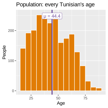
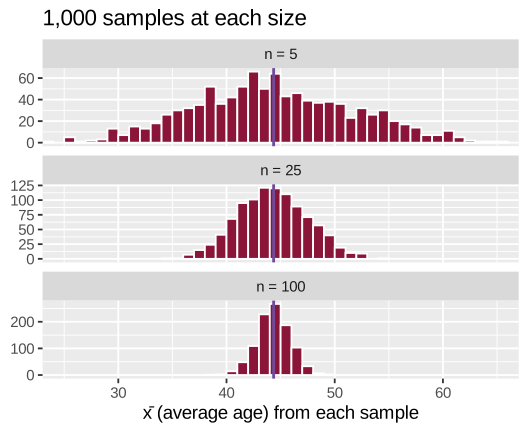
Sample size is important!

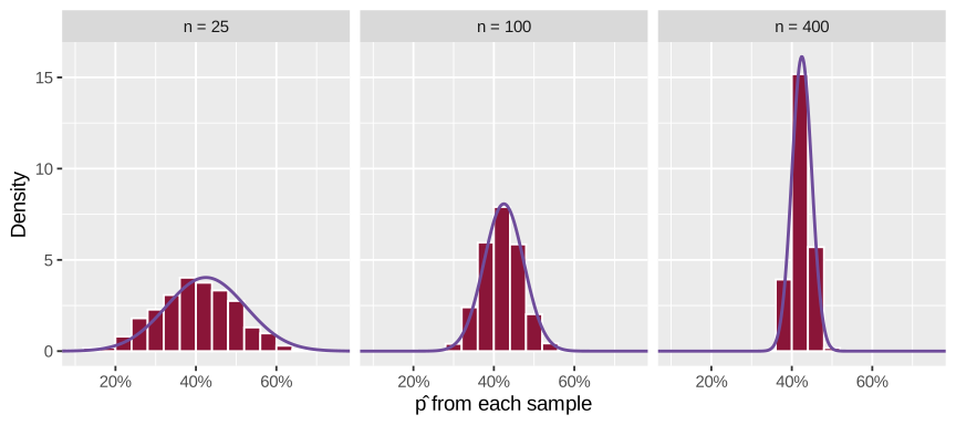
Two kinds of spread

Standard deviation

How much do individual values vary?

How different is one Tunisian from another?

For yes/no data:

\sqrt{p(1 - p)} = 0.494

Standard error

How much do sample statistics vary?

How different is one sample’s \widehat{p} from another’s?

The standard deviation of the sampling distribution

Standard error formula

\text{SE}(\widehat{p}) = \frac{\text{SD}}{\sqrt{n}} = \sqrt{\frac{p (1 - p)}{n}}

Sample size	SE from 1,000 samples	SE from formula
25	0.1	0.099
100	0.047	0.049
400	0.022	0.025

The formula matches the simulations!
Bigger n → smaller SE
\sqrt{n} means 4× the people → ½ the SE

Bigger samples don’t fix bias

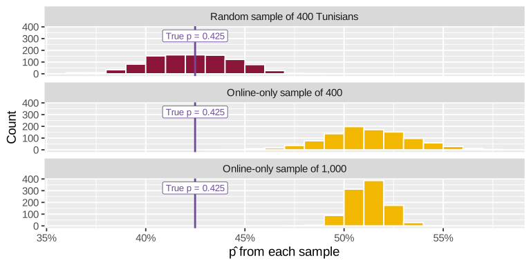
Random sampling puts the center in the right place; sample size controls the width

Uncertainty

Trump’s approval rating is 34.9% (+/-2.1% pts.)

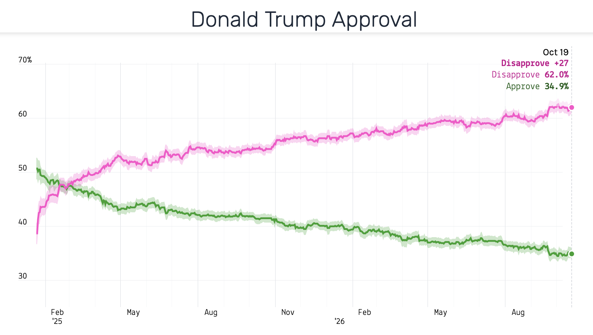
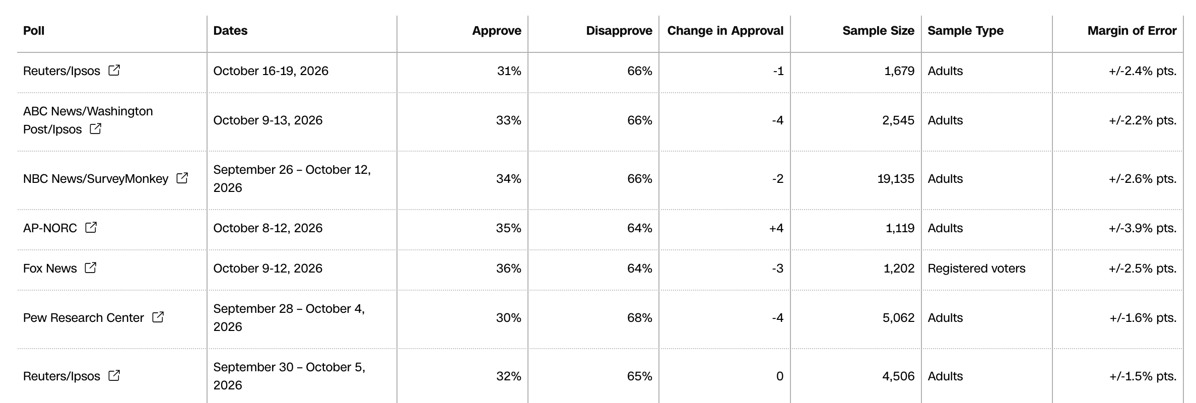
How accurate is the estimate?

In real life we only get one sample
We can’t see the whole sampling distribution—we don’t know the true population parameter
But the CLT tells us what the sampling distribution looks like…

Normal curves have rules

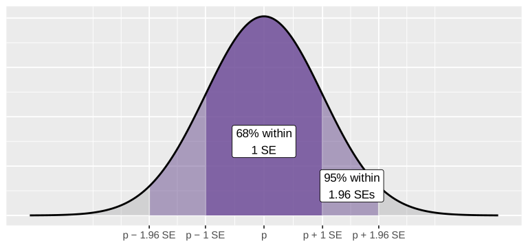
Our 1,000 samples of 100: 70% within 1 SE of p; 96.5% within 1.96 SEs

Flip it around

95% of \widehat{p}s are within 1.96 SEs of p
So if we reach 1.96 SEs out from our \widehat{p} in both directions, we’ll catch the true p in 95% of samples

Margin of error

How far to reach

\text{MOE} = 1.96 \times \text{SE}

(≈ 2 × SE)

Confidence interval

The range you get

\widehat{p} \pm \text{MOE}

(a 95% confidence interval)

\text{SE} \approx \sqrt{\frac{\widehat{p} (1 - \widehat{p})}{n}}

40 out of 100 Tunisians have thought about emigrating

\widehat{p} = 0.4
\text{SE} \approx \sqrt{\frac{0.4 \times 0.6}{100}} = 0.049
\text{MOE} = 1.96 \times 0.049 = 0.096
40% ± 9.6 points → 30.4% to 49.6%

The true p (42.5%) is in there!

\text{SE} \approx \sqrt{\frac{\widehat{p} (1 - \widehat{p})}{n}}

400 out of 1,000 Tunisians have thought about emigrating

\widehat{p} = 0.4
\text{SE} \approx \sqrt{\frac{0.4 \times 0.6}{1000}} = 0.0155
\text{MOE} = 1.96 \times 0.0155 = 0.0304
40% ± 3.0 points → 37.0% to 43.0%

The true p (42.5%) is still in there!
(but now the estimate is narrower and more precise)

100 samples, 100 intervals

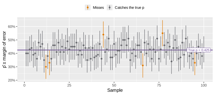
94 of these 100 intervals include the true p

What does “95% confidence” mean?

If we took sample after sample and made an interval each time, about 95% of those intervals would include the true p
The 95% describes the method, not any single interval
Our one interval either caught p or it didn’t—we just can’t know which
Bigger samples → narrower intervals, but still 95% of them catch the truth

Much more about confidence intervals in ModernDive chapter 8!

Back to the poll

Trump’s approval rating is 34.9% (+/-2.1% pts.)

Point estimate: \widehat{p} = 34.9%
Margin of error: ± 2.1 points
95% confidence interval: 32.8% to 37.0%

Approval is plausibly anywhere from about 33% to 37%

MOE isn’t perfect

The margin of error only measures sampling variation, not these:

Biased samples (online-only surveys!)
Non-response
People who refuse to answer
Confusing or leading questions
People who lie or give the “polite” answer

Emigration, with margins of error

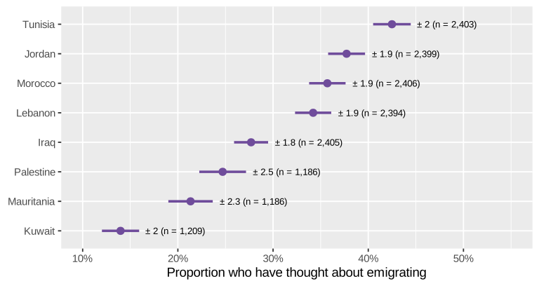
Our M&Ms, with a margin of error

Back to Positron!

Calculate the SE and margin of error for your own bag’s \widehat{p}_\text{green}
Calculate the SE and margin of error for the class’s pooled \widehat{p}_\text{green}
Which one is more useful? Why?

Choosing a
sample size

How many people do we need?

It depends on three things

Precision: How big of a margin of error can you live with?
Confidence: How sure do you want to be? (95% → 1.96)
Variability: How spread out are the answers? (p(1 - p))

Notice what’s not on the list: how big the population is!

Flip the formula

\text{MOE} = 1.96 \times \sqrt{\frac{p (1 - p)}{n}} \quad \rightarrow \quad n = \frac{1.96^2 \times p (1 - p)}{\text{MOE}^2}

But we don’t know p before we survey anyone!
Play it safe: p(1 - p) is biggest when p = 0.5
That gives you the biggest (worst-case) sample size

Example: ± 3 points

We want a margin of error of 3 percentage points (0.03)
Assume the worst: p = 0.5
n = \frac{1.96^2 \times 0.5 \times 0.5}{0.03^2} = \frac{0.9604}{0.0009} = 1,067.1
Always round up: 1,068 people

That’s why so many polls survey ≈1,000 people

Quick rule of thumb

1.96^2 \times 0.5 \times 0.5 \approx 1, so:

Margin of error from n

\text{MOE} \approx \frac{1}{\sqrt{n}}

n = 1,000 → \frac{1}{\sqrt{1000}} = ± 3.2 points

n from margin of error

n \approx \frac{1}{\text{MOE}^2}

± 3 points → \frac{1}{0.03^2} ≈ 1,111 people

Precision is expensive

Margin of error	People needed	Cost at QAR 50 per interview
± 10 points	97	QAR 4,850
± 5 points	385	QAR 19,250
± 3 points	1,068	QAR 53,400
± 2 points	2,401	QAR 120,050
± 1 points	9,604	QAR 480,200

Cut the margin of error in half → 4× the people

Diminishing returns

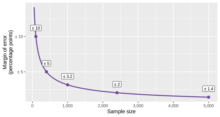
Most national surveys stop at ≈1,000–2,500 people

Population size doesn’t matter

± 3 points needs ≈1,068 people in Qatar (≈3 million), Tunisia (≈12 million), or the United States (≈340 million)
Soup!

Subgroup sizes

All Tunisians (n = 2,403): 42% have thought about emigrating, ± 2 points
Young Tunisians, 18–29 (n = 482): 70%, ± 4.1 points
Want ± 3 points for young people? You need ≈1,068 young people

Plan your sample size around the smallest group you care about

Surveys often oversample small groups (and use weights to fix the overall results)

Using what you already know

p = 0.5 is the worst case
If past surveys (or M&M bags!) tell you p is around 0.17, use that instead
0.5 \times 0.5 = 0.25, but 0.17 \times 0.83 ≈ 0.14
± 3 points with p = 0.17: 603 people instead of 1,068

Your turn: how many M&Ms?

Assume p_\text{green} ≈ 0.17 (our class’s estimate) and each bag has ≈50 M&Ms

n = \frac{1.96^2 \times p (1 - p)}{\text{MOE}^2}

How many M&Ms do you need to estimate p_\text{green} within ± 5 points? How many bags is that?
How many M&Ms for ± 2 points? How many bags?
How many bags did our class have? Was that enough?

How many M&Ms?

± 5 points: \frac{1.96^2 \times 0.17 \times 0.83}{0.05^2} = 217 M&Ms ≈ 5 bags
± 2 points: \frac{1.96^2 \times 0.17 \times 0.83}{0.02^2} = 1,356 M&Ms ≈ 28 bags

One bag can’t tell the factories apart—but a whole class can!

Beyond proportions

Means: n = \left(\frac{1.96 \times \sigma}{\text{MOE}}\right)^2
- Need a guess for the standard deviation \sigma (from past studies or a small pilot survey)
Differences and regression slopes: “power analysis”
- How many people do I need to detect an effect of a certain size?
- Often easiest to figure out with simulation—the same trick we used today!

Sampling I & II

Plan for today

Populationsand samples

Data so far

The Arab Barometer

Thought about emigrating?

Population vocabulary

Counting the population

Measuring the sample

Parameters and statistics

Is the sample any good?

M&Ms

M&M colors!

What about Qatar?

Mars Polska

Your bag is a sample

Define the population

Census or sample?

Your turn: count your bag

Is your bag a good sample?

What could go wrong?

Who’s right?

Getting a better estimate

Our class’s estimate

What did we find?

Plan for today

Sampling variation

What our bags taught us

We can’t buy 1,000 bags

Simulation

A virtual vat

1,000 virtual bags

Repeat 1,000 times

Sampling distribution

Three different distributions

More samples or bigger samples?

Central limit theorem

It works for averages too

Sample size is important!

Two kinds of spread

Standard error formula

Bigger samples don’t fix bias

Uncertainty

How accurate is the estimate?

Normal curves have rules

Flip it around

100 samples, 100 intervals

What does “95% confidence” mean?

Back to the poll

MOE isn’t perfect

Emigration, with margins of error

Our M&Ms, with a margin of error

Choosing asample size

How many people do we need?

Flip the formula

Example: ± 3 points

Quick rule of thumb

Precision is expensive

Diminishing returns

Population size doesn’t matter

Subgroup sizes

Using what you already know

Your turn: how many M&Ms?

How many M&Ms?

Beyond proportions

Populations
and samples

Choosing a
sample size