Estimation, confidence intervals, and bootstrapping

Quantitative Methods for
International Politics

IPOL 3270 • Fall 2026

November 1, 2026

Plan for today

Quick review so far

Estimands

Bootstrapping

Quick review

Inference stuff so far

Inference = using a sample to say something about the population

In the flavor of statistics we’re doing, there’s a true, fixed population parameter out in the world

• It exists whether or not we ever collect any data
• It doesn’t move around—the samples do
• We can’t measure it directly, so we make inferences

Bouncing values

• We can’t measure everything, so we take one sample and calculate a statistic (\widehat{p}, \bar{x}, a median, a slope)
• Individual values in that sample vary and bounce around the average = standard deviation
• A different sample would give a different statistic = sampling variation
• So how far off might our statistic be from the population parameter?

SE and confidence

• With lots of samples, the statistics would form a sampling distribution
• The standard deviation of that distribution is the standard error
• Statistic ± 1.96 × SE gives a 95% confidence interval

Sampling distributions

But we only have one sample, so we can’t see the sampling distribution!

Assume its shape

Math: CLT says it should be normal, so use SE formulas

Simulate it

Bootstrapping: resample our sample a bunch of times

Plan for this week

1. What do we actually measure? Which summary statistic answers our research question?
2. How do we get the standard error?
3. How do confidence intervals actually work? (next time!)

Estimands

Every quantitative study has to answer one question

What is your estimand?

Estimand

The thing you want to know

The population parameter

Estimator

The method for guessing it

A formula or procedure you apply to a sample

Estimate

The number you get

The result from one specific sample

You’ve already done this!

	M&Ms	Tunisia
Estimand	p_\text{green}: proportion of green M&Ms made in Janaszówek	p: proportion of all Tunisian adults who have thought about emigrating
Estimator	Green M&Ms ÷ all M&Ms in a sample from Carrefour	“Yes” answers ÷ all answers in a random sample
Estimate	\widehat{p}_\text{green} = 0.17	\widehat{p} = 0.425

Lots of possible estimands

Estimand	Parameter	Statistic	Example
Proportion	p	\widehat{p}	Tunisians who have thought about emigrating
Mean	\mu	\bar{x}	Average age of Tunisian adults
Median	m	\widehat{m}	Typical number of countries visited
Difference in proportions	p_1 - p_2	\widehat{p}_1 - \widehat{p}_2	Emigration: internet users vs. non-users
Difference in means	\mu_1 - \mu_2	\bar{x}_1 - \bar{x}_2	Democracy score: GCC vs. non-GCC countries
Regression slope	\beta_1	b_1	Relationship between age and thinking about emigrating

Estimand = quantity + population

“Do people in the Arab world
want to leave?”

• Who? Adults? Young people? Which countries? When?
• What? Ever thought about it? Have plans? Actually applied for a visa?
• What number? Proportion? Difference between groups?

Proportion of all Tunisian adults in 2023–24 who say they’ve thought about emigrating

No single correct estimand!

Is thinking about emigrating more common among young Tunisians?

Estimand	Estimate	What it tells us
p_\text{young} - p_\text{older}	34.8 points	Gap between people 18–29 and everyone older
Slope of age, \beta_1	-1.2 points per year	How the chance changes with each extra year of age

Same question, different numbers! Decide which one matches your question before you calculate anything

Your turn: define the estimand

1. Do women trust their governments more than men do?
2. Do young people care more about democracy?
3. Does corruption lead to worse human rights?
4. Do mosquito nets improve public health?

For each one:

• Population: Who exactly are we talking about?
• Quantity: Proportion? Mean? Median? Difference?
• Statistic: What would you calculate?

Bootstrapping

Measuring sampling variation

Simulation

Our virtual vat of M&Ms, our pretend Tunisia

But you need the whole population. If you had it, you wouldn’t need a sample!

Math

\text{SE} = \sqrt{\frac{\widehat{p} (1 - \widehat{p})}{n}}

But you need a formula, and a friendly formula doesn’t exist for everything

What’s the standard error of a median?

(or any of these estimands, really?)

Improvise!

• We only have one sample
• Our best guess about the population is… our sample!
• So use the sample as a pretend population and take samples from it

Bootstrapping: using the sample you have to make lots of new samples

How to bootstrap

1. Take a bootstrap sample

   Sample with replacement, same size as the original

2. Calculate a statistic from that bootstrap sample

   Mean, median, proportion, difference, slope, whatever

3. Repeat a bunch of times

   1,000 times or more

4. Look at all the statistics

   That’s the bootstrap distribution

What resampling looks like

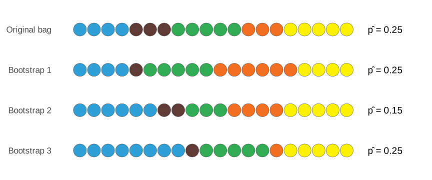
Some M&Ms show up twice or more and some don’t show up at all, so \widehat{p} changes from resample to resample

Our turn: class sample

How many countries has a typical GU-Q student been to?

• Population
• Quantity
• Statistic

Write how many countries you’ve been to on the board

Our estimate

library(tidyverse)
library(moderndive)

# Numbers from the board
countries <- tibble(
  n_countries = c(8, 11, 21, 4, 23, 19, 16,
                  11, 5, 3, 4, 8, 8, 16, 30,
                  8, 9, 10, 11, 12, 13)
)

countries |>
  summarize(stat = median(n_countries))

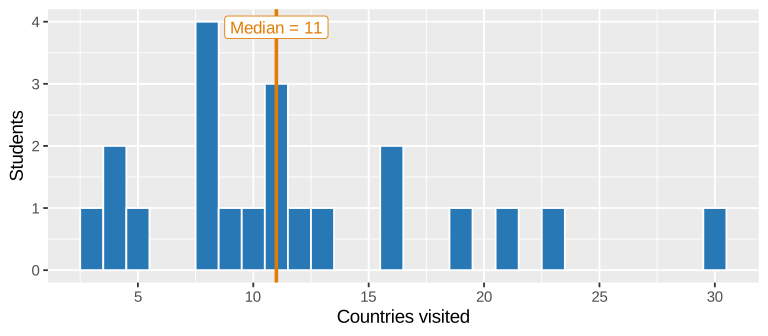
ggplot(countries, aes(x = n_countries)) +
  geom_histogram(binwidth = 1, color = "white")

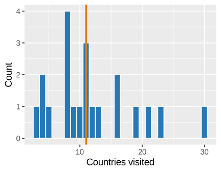
Median = 11

Does this reflect all of GU-Q? How confident are we that this number is right? We don’t know what the sampling distribution looks like!

Your turn: bootstrap by hand

How many countries has a typical GU-Q student been to?

1. Go to random.org on your phone
2. Generate a random number between 1 and 21
3. Write down that observation’s number of countries on your paper
4. Generate another random number, write that down, and repeat
5. Find the median of your random 21 numbers
6. Write that median on the board

Plan for today

Bootstrapping, continued

Confidence intervals

Comparing with intervals

Estimand

The thing you want to know

The population parameter

Estimator

The method for guessing it

A formula or procedure you apply to a sample

Estimate

The number you get

The result from one specific sample

	M&Ms	Tunisia
Estimand	p_\text{green}: proportion of green M&Ms made in Janaszówek	p: proportion of all Tunisian adults who have thought about emigrating
Estimator	Green M&Ms ÷ all M&Ms in a sample from Carrefour	“Yes” answers ÷ all answers in a random sample
Estimate	\widehat{p}_\text{green} = 0.17	\widehat{p} = 0.425

Goal of inference

Make a good enough guess about the true population parameter

How do we know if the guess is good?

How confident are we that we captured the actual population parameter?

Variability

Every sample statistic (mean, median, correlation, slope, etc.) has some variability

If we take a bunch of samples, that statistic will bounce around

We can measure that variability with math or simulation

Our sample

21 students; typical student has been to 11 countries

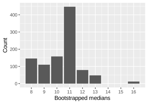
Our bootstrapped medians

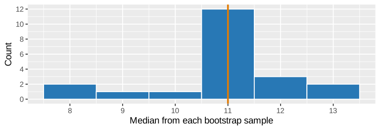
• What shape do our medians make? Where’s the center?
• Does this range tell us about all GU-Q students?

Bootstrapping tells us about sampling variation—
it doesn’t create a random sample!

Lots of bootstraps

set.seed(1234)
boot_countries <- countries |>
  rep_slice_sample(
    n = nrow(countries),
    replace = TRUE,
    reps = 1000
  ) |>
  summarize(stat = median(n_countries))

ggplot(boot_countries, aes(x = stat)) +
  geom_histogram(binwidth = 1, color = "white")

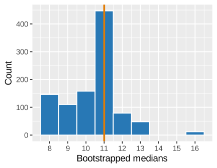
1,000 medians instead of our handful on the board. Lumpy, because a median of whole numbers can only land on a few values!

The {infer} way

library(infer)

boot_countries <- countries |>
  specify(response = n_countries) |>
  generate(
    reps = 1000,
    type = "bootstrap"
  ) |>
  calculate(stat = "median")

• specify(): What’s the variable?
• generate(): Make the bootstrap samples
• calculate(): Find the statistic for each one

The {infer} way

boot_countries

Response: n_countries (numeric)
# A tibble: 1,000 × 2
   replicate  stat
       <int> <dbl>
 1         1    12
 2         2    11
 3         3    11
 4         4    11
 5         5    11
 6         6    11
 7         7    11
 8         8    11
 9         9     8
10        10    11
# ℹ 990 more rows

visualize(boot_countries)

Same idea as the rep_slice_sample() version: one row per bootstrap sample, with its median in stat. visualize() is just a shortcut for a ggplot histogram.

Seeds

# Choose 5 numbers between 1 and 100
sample(1:100, 5)

[1] 14 51 80 90 92

 

# Do it again
sample(1:100, 5)

[1] 24 58 93 75 96

Seeds

# Choose 5 numbers between 1 and 100
set.seed(1234)
sample(1:100, 5)

[1] 28 80 22  9  5

 

# Do it again
set.seed(1234)
sample(1:100, 5)

[1] 28 80 22  9  5

Seeds

A seed lets you make the same random numbers every time you run your code

Any whole number

set.seed(1)
set.seed(13)
set.seed(42)
set.seed(1234)
set.seed(12345)
set.seed(20261101)

Median GDP per capita

library(tidyverse)
library(moderndive)
library(infer)

# The statistic from our actual data
obs_median <- un_member_states_2024 |>
  specify(response = gdp_per_capita) |>
  calculate(stat = "median")

# The bootstrap distribution
set.seed(1234)
boot_median <- un_member_states_2024 |>
  specify(response = gdp_per_capita) |>
  generate(reps = 1000, type = "bootstrap") |>
  calculate(stat = "median")

visualize(boot_median) +
  geom_vline(xintercept = obs_median$stat)

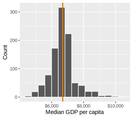
Mean: $18,177
Median: $6,696

GDP per capita is really skewed, so the median describes a typical country better than the mean, and there’s no friendly SE formula for it. The warning about a removed row is just infer dropping a country with missing GDP.

This is every UN member, not a random sample, so it’s worth asking what the population even is here. One answer: think of this year’s countries as one draw from all the ways the world could have turned out. Ages from the Arab Barometer are a real sample, but their medians get stuck on one or two whole numbers.

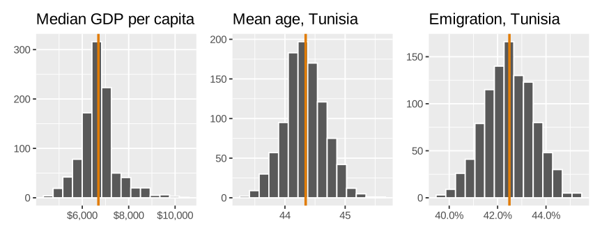
Works for any estimand!

# Mean age
boot_mean <- tunisia |>
  specify(response = age) |>
  generate(
    reps = 1000,
    type = "bootstrap"
  ) |>
  calculate(stat = "mean")

# Thought about emigrating
boot_emigrate <- tunisia |>
  drop_na(thought_emigrating) |>
  specify(
    response = thought_emigrating,
    success = "Yes"
  ) |>
  generate(
    reps = 1000,
    type = "bootstrap"
  ) |>
  calculate(stat = "prop")

drop_na() is required here. With missing values in a yes/no column, calculate() stops with an error saying a proportion isn’t well defined for a “multinomial” response.

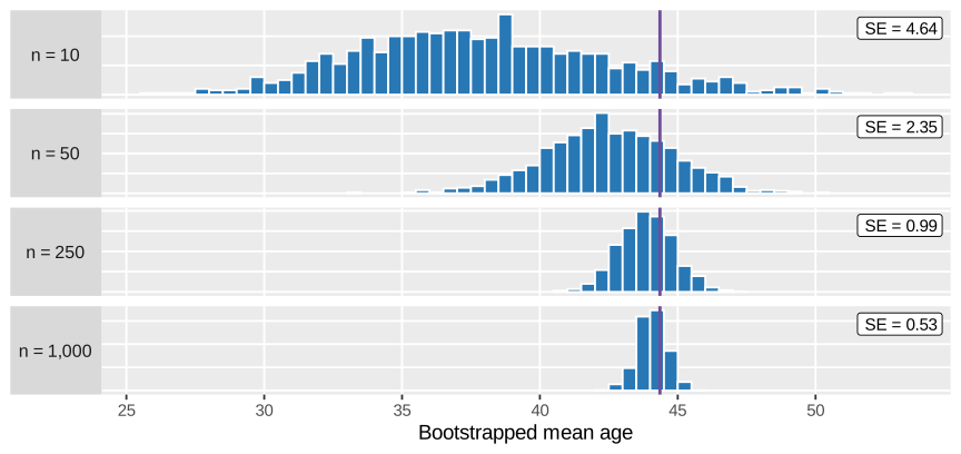
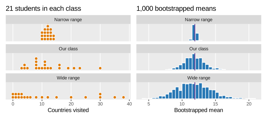
A bootstrap distribution only knows what’s in your sample

• More observations → less bouncing around
• More spread in the sample → more bouncing around

More observations

n = 10 is wide and a little lopsided; n = 1,000 is a narrow bell. 4× the people → ½ the SE again (250 → 1,000).

The n = 10 sample happened to get young people, so its distribution is centered way below the truth. Bootstrapping can’t fix an unlucky sample—it centers on whatever your sample says.

More spread

Math or bootstrap?

Math

• Fast, built in to everything
• Needs a formula
• Needs assumptions (like normality) to be okay
• It’s what you’ll see in most published research

Bootstrap

• Works for almost any statistic
• Needs a computer
• Still needs a good sample
• Struggles with tiny samples and statistics at the extremes

When both work, they should give you about the same answer

Quick demo if there’s time: bootstrap the largest value with summarize(stat = max(age)). A resample can never beat the sample’s maximum, so most of the bootstrap distribution piles up on one number.

So why even do this?

Most published research reports math-based standard errors

Intuition!

• Every math-based SE in a regression table is a shortcut for one of these histograms
• Formulas are the mathy way of guessing what the bootstrap distribution would look like

Confidence intervals

Spear or net?

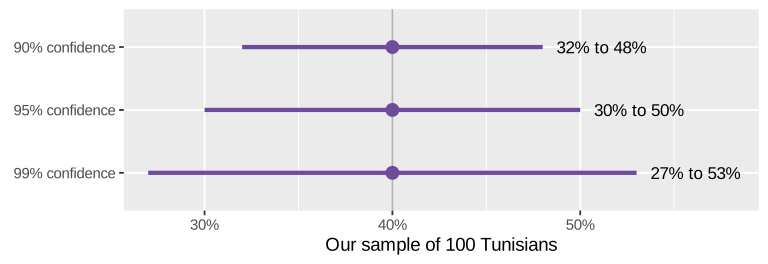
Point estimate

Fishing with a spear

One number: \widehat{p} = 0.4

Almost certainly misses by a little

Interval estimate

Fishing with a net

A range: 30% to 50%

Much better chance of catching the fish

How wide should the net be? It depends on the sampling variation

The Range Game

Round 1

Write a range that’s exactly as wide as your window. No phones!

Example: a window 10 years wide → (1630 to 1640)

1. How many time zones does Russia have? Window: 2
2. How many members does the Arab League have? Window: 4
3. How tall is the Burj Khalifa, in meters? Window: 50 meters
4. In what year did the Suez Canal open? Window: 10 years
5. How many goals were scored in the 2022 World Cup in Qatar? Window: 20 goals

~20 seconds per question. Make sure people are actually using the exact width: (1630 to 1640), not (1600 to 1700).

Round 1 answers

1 point for each window that caught the answer

1. Russian time zones: 11
2. Arab League: 22
3. Burj Khalifa: 828 m
4. Suez Canal: 1869
5. 2022 World Cup goals: 172

Round 2

6. In what year was Georgetown University founded? Window: 100 years
7. How many members does the African Union have? Window: 30
8. How long is the Nile, in kilometers? Window: 3,000 km
9. How many members does the Organisation of Islamic Cooperation have? Window: 30
10. How tall is Mount Everest, in meters? Window: 3,000 meters

Round 2 answers

6. Georgetown: 1789
7. African Union: 55
8. Nile: ~6,650 km
9. Organisation of Islamic Cooperation: 57
10. Mount Everest: 8,849 m

Round 3

Choose your own range!

Question	3 points if width ≤	2 points if width ≤	1 point if wider
11. In what year was the Universal Declaration of Human Rights adopted?	2 years	10 years	✓
12. In what year was the Kingdom of Saudi Arabia founded?	2 years	10 years	✓
13. How big is Qatar, in square kilometers?	1,000 km²	3,000 km²	✓
14. How long is the Suez Canal, in kilometers?	10 km	50 km	✓
15. How many countries are parties to the Convention on the Rights of the Child?	10 countries	50 countries	✓

Round 3 answers

11. Universal Declaration of Human Rights: 1948
12. Kingdom of Saudi Arabia: 1932
13. Qatar: 11,581 km²
14. Suez Canal: 193 km
15. Convention on the Rights of the Child: 196

How did the windows do?

• Why did the wide windows catch more than the narrow windows?
• If you were a contestant on the show, what size window would you want? What about the show’s producer?
• In Round 3, how did you decide your widths?
• Why not make every net as wide as possible?

Wider nets catch more
but tell you less!

Possible answers (adapted from Grosofsky):

• Contestant: as wide as possible, so you always win. A window covering every possible price is 100% confident.
• Producer: narrow, so nobody wins and prizes are cheap; or medium, so enough people win to keep the show fun. Someone probably calculated the win rate for different widths.
• Round 3: people go narrow on questions they know well (UDHR? Saudi Arabia?) and wide on ones they don’t (Suez length? Qatar’s area?). Knowing less is like having a smaller or noisier sample—you need a wider net to catch the truth just as often.
• Widest possible: “the UDHR was adopted between 1000 and 2100” is never wrong and totally useless, like the Garfield forecast coming up.

From distribution to interval

A plausible range of values for the true population parameter

• We have a bootstrap distribution
• It shows how much a statistic bounces around
• Two ways to turn it into a range: the standard error method and the percentile method

Standard error method

The bootstrap distribution’s standard deviation is the standard error, so plug it in to the same equation from last week

\widehat{p} \pm 1.96 \times \text{SE}_\text{bootstrap}

0.4 \pm 1.96 \times 0.049

30.4% to 49.6%

Only works when the bootstrap distribution is bell-shaped!

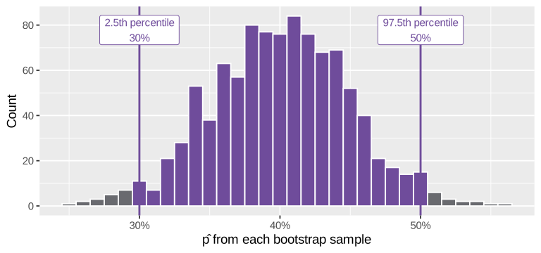
Percentile method

Skip the standard error: a 95% confidence interval is the middle 95% of the bootstrap distribution

How do they compare?

Method	Lower	Upper
Bootstrap: standard error	30.4%	49.6%
Bootstrap: percentile	30.0%	50.0%
Last week: formula	30.4%	49.6%

When the distribution is bell-shaped, they’re basically identical!

Which one should I use?

Standard error

Needs a bell-shaped distribution

Good for proportions, means, differences, and slopes

Helps show where the formulas come from

Percentile

Works for almost any statistic

Good for lumpy or skewed distributions, like our medians

Median age: 39 to 50

Our median countries: 8 to 13

With {infer}

boot_green |>
  get_ci(level = 0.95, type = "se", point_estimate = class_p_green)

boot_green |>
  get_ci(level = 0.95, type = "percentile")

Method	lower_ci	upper_ci
Standard error	0.149	0.192
Percentile	0.149	0.193

95% confidence intervals for our M&Ms’ \widehat{p}_\text{green}

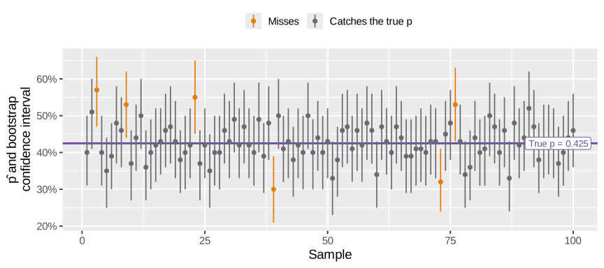
What does “95%” mean?

• The true p is fixed; the intervals move around
• About 95% of intervals made this way catch the true p
• The 95% describes how we make the interval, not one specific interval
• A specific interval either caught p or it didn’t—we just can’t tell which

Don’t be tempted!

Tempting, but wrong

“There’s a 95% chance that the true p is between 30% and 50%”

People do this all the time! People with PhDs! You will too!

Legal and correct

“There’s a 95% chance that the interval (30%, 50%) captures the true p”

“We’re 95% confident the interval (30%, 50%) captures the true p”

One random sample of 94 Tunisians gives a 95% confidence interval for the median age of 39 to 50.

A. 95% of Tunisians in this sample have a median age between 39 and 50

B. 95% of all Tunisians are between 39 and 50 years old

C. We’re 95% confident that the median age of all Tunisians is between 39 and 50

D. We’re 95% confident that the median age in this sample is between 39 and 50

C! The interval is about the population’s median, not individual people and not our sample

A pollster surveys a random sample of 800 Jordanians and finds a 90% confidence interval for the proportion who trust their government.

A. If they ran many identical polls, about 90% of the intervals would capture the true proportion

B. About 90% of Jordanians who trust their government would respond to the poll

C. If they repeated the poll 20 times, about 18 of the intervals would capture the true proportion

D. There’s a 90% chance that the true proportion is in this specific interval

A and C! D is tempting, but wrong

Imagine a planner takes a random sample of 200 apartment listings in Doha and calculates a 95% confidence interval for average rent: QAR 15,000 to QAR 27,000.

A. If they took another sample of 200, there’s a 95% chance its mean would be between QAR 15,000 and QAR 27,000

B. About 95% of the apartments in the sample rent for QAR 15,000 to QAR 27,000

C. We’re 95% confident that the interval captured the true average rent

D. There’s a 95% chance that the true average rent is between QAR 15,000 and QAR 27,000

C!

What level should I use?

• 90%, 95%, and 99% are the most common
• Want to be more confident you got the p? Use a bigger net or wider window!

Getting a narrower net

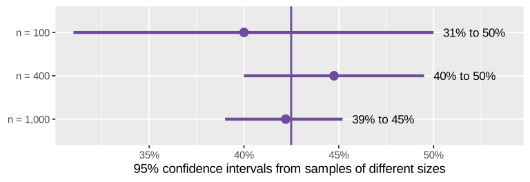
• Lower confidence → narrower, but more misses
• Bigger sample → narrower, with the same confidence

Comparing with intervals

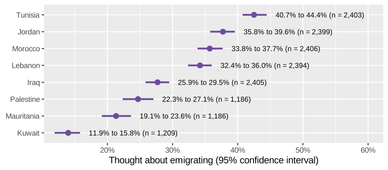
• Which countries are clearly higher or lower than Tunisia? Which ones can’t we tell apart?
• Why are Mauritania’s and Palestine’s nets wider than Iraq’s?
• Kuwait has a small sample too, but its net isn’t wide. Why not?

Mauritania and Palestine have half as many people as Iraq → wider. Kuwait has ~1,200 people too, but with p̂ near 0.14 there’s less variation to bounce around (p(1 − p) is small near 0 or 1), so its width roughly matches Tunisia’s.

Careful with overlap: nets that don’t overlap are clearly different, but slightly overlapping nets can still be significantly different. The real way to check is an interval for the difference, coming up next.

Differences between groups

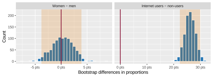
Are Tunisian women more likely to have thought about emigrating than men?

boot_gender <- tunisia |>
  drop_na(thought_emigrating) |>
  specify(thought_emigrating ~ gender, success = "Yes") |>
  generate(reps = 1000, type = "bootstrap") |>
  calculate(stat = "diff in props", order = c("Female", "Male"))

• Estimand: p_\text{women} - p_\text{men}
• Works the same with "diff in means"

0.1 points (-3.8 to 3.9)

Includes 0: no difference is plausible

26.1 points (22.3 to 29.9)

Way above 0: no difference is not plausible

Careful wording: an interval that includes 0 means 0 is plausible, NOT that the groups are equal. This is the setup for hypothesis testing next week.

We can stop ignoring these!

model <- lm(yes_num ~ age, data = tun_ages)
get_regression_table(model)

term	estimate	std_error	statistic	p_value	lower_ci	upper_ci
intercept	0.9755	0.0275	35.5153	0	0.9217	1.0294
age	-0.0124	0.0006	-21.2940	0	-0.0135	-0.0112

• Each extra year of age → 1.2 point lower chance of having thought about emigrating
• lower_ci and upper_ci are a 95% confidence interval from a formula
• Bootstrapping with calculate(stat = "slope"): -0.0133 to -0.0114

Moral of the story

• Always define an estimand: what do you want to know, and about whom?
• Sample statistic ≠ population parameter, but a good sample gets close
• We can’t keep sampling from the population, so we bootstrap
• Bootstrapping measures uncertainty; it doesn’t improve your estimate or fix a biased sample
• Report estimates with confidence intervals