Hypothesis testing

Quantitative Methods for
International Politics

IPOL 3270 • Fall 2026

November 8, 2026

Plan for today (and Tuesday)

Evidentiary standards

How to test any hypothesis

Interpreting tests

Other δs

Math-based tests

Problems with p-values

Quick review

Estimands

Parameters are the things we
want to know about the population

Estimand Parameter Statistic Example
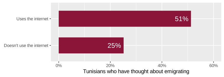
Proportion p \widehat{p} Tunisians who have thought about emigrating
Mean \mu \bar{x} Average age of Tunisian adults
Difference in proportions p_1 - p_2 \widehat{p}_1 - \widehat{p}_2 Emigration: internet users vs. non-users
Difference in means \mu_1 - \mu_2 \bar{x}_1 - \bar{x}_2 Age: urban vs. rural residents
Regression slope \beta_1 b_1 Relationship between age and thinking about emigrating

  • \widehat{p}
  • \bar{x}
  • \widehat{p}_1 - \widehat{p}_2
  • \bar{x}_1 - \bar{x}_2
  • b_1

\delta

(delta)

Your estimate

Whatever statistic answers your research question

How do we know if δ is any good?

Is it accurate?

Is δ a good guess?

Did it pick up the population parameter?

Confidence intervals

Is it real?

Is δ real?

Could it maybe be zero?

Hypothesis tests and p-values

Is it substantive?

Does δ even matter?


Your knowledge of the world—no stats!

Do different groups of Tunisians think about emigrating at different rates?

Comparison δ 95% CI
Women − men 0.1 points -3.8 to 3.9
Internet users −
non-users
26.1 points 22.3 to 29.9
  • The gender interval includes 0, so “no difference” is plausible
  • The internet interval is way above 0
  • Is there a more formal way to ask “could it be zero”?

Evidentiary standards

Common law evidentiary standards

  • Preponderance of the evidence (civil)
  • Clear and convincing evidence (civil)
  • Beyond a reasonable doubt (criminal)

Sharia court evidentiary standards

  • غلبة الظن / preponderance of assumption (ta’zir and family matters)
  • اليقين / certainty (hudud and qisas cases)

  • Why do we have all these levels?
  • Why is the burden different for different types of cases?
  • Why is it so high for criminal cases?

We’re afraid of punishing an innocent person!

“For if the Imam makes a mistake in forgiving it would be better than making mistake in punishment”

Jamiʿ at-Tirmidhi 1424

فَإِنَّ الإِمَامَ أَنْ يُخْطِئَ فِي الْعَفْوِ خَيْرٌ مِنْ أَنْ يُخْطِئَ فِي الْعُقُوبَةِ

جامع الترمذي 1424

Two possible hypotheses

Is there a difference between men’s and women’s attitudes toward emigration in Lebanon?

Null hypothesis

H_0: p_\text{women} - p_\text{men} = 0

No difference (“innocent”)

Alternative hypothesis

H_A: p_\text{women} - p_\text{men} \neq 0

Some difference (“guilty”)

α (alpha)

0.10
0.05
0.01

Your evidentiary standard: how often you’re willing to make a Type I error

Statistical significance

There’s enough evidence to safely declare that δ is “real” and not zero

“Rejecting the null hypothesis”

p-values

The probability of seeing a δ at least that extreme in a world where there’s no effect

Wildly misunderstood—by everyone!

How to test
any hypothesis

There is only one test!

Simulations and null worlds

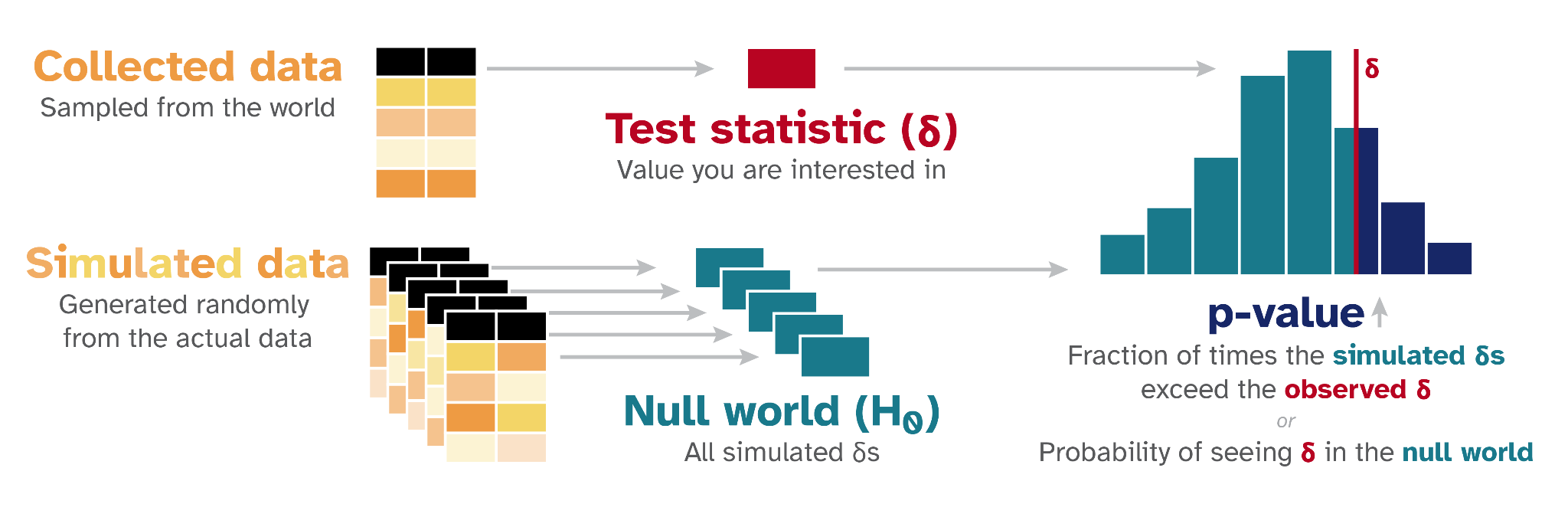
Diagram of the one test: collected data gives a test statistic δ; simulated data gives a null world of many δs; the p-value is the fraction of simulated δs that exceed the observed δ

Diagram of the one test, revealed one piece at a time: collected data, then the test statistic δ, then simulated data, then the null world of simulated δs, then the histogram of the null world with δ marked, then the p-value

1: Find δ

2: Invent a world where δ is null

3: Look at δ in the null world

4: Find the probability that δ could exist in the null world

5. Decide!

1: Calculate δ

Do Lebanese women and men think about emigrating at different rates?

  • Estimand: p_\text{women} - p_\text{men}
  • H_0: p_\text{women} - p_\text{men} = 0
  • H_A: p_\text{women} - p_\text{men} \neq 0
  • α = 0.05
Gender % yes n
Women 32.3% 1,188
Men 36.1% 1,206

δ = -3.7 points

Is that real though? Could it be positive? Could it be zero?

2: Invent a world where δ is null

If gender doesn’t matter, the categories “woman” and “man” are meaningless

  • Shuffle them!
    • Keep everyone’s answers, but randomly reassign who’s a woman and who’s a man
    • (“permutation shuffling” breaks any connection between the variables)
  • Calculate δ for the shuffled data
  • Repeat a bunch of times

Bootstrapping vs. permuting

Bootstrap

Resample with replacement

Shows how much δ bounces around

type = "bootstrap"

→ Confidence intervals

Permutation

Shuffle without replacement

Shows what δ looks like when there’s no effect

type = "permute"

→ Hypothesis tests

library(infer)

# δ from the actual data
obs_diff <- lebanon |>
  specify(
    thought_emigrating ~ gender,
    success = "Yes"
  ) |>
  calculate(
    stat = "diff in props",
    order = c("Female", "Male")
  )

# Simulate null world
null_world <- lebanon |>
  specify(
    thought_emigrating ~ gender,
    success = "Yes"
  ) |>
  hypothesize(null = "independence") |>
  generate(reps = 1000, type = "permute") |>
  calculate(
    stat = "diff in props",
    order = c("Female", "Male")
  )
  • specify(): What are the variables?
  • hypothesize(): What does the null world look like? ("independence" = gender and emigration aren’t related)
  • generate(): Make the null world by shuffling ("permute")
  • calculate(): Find δ in each shuffled dataset

null_world
Response: thought_emigrating (factor)
Explanatory: gender (factor)
Null Hypot...
# A tibble: 1,000 × 2
   replicate     stat
       <int>    <dbl>
 1         1  0.0177 
 2         2  0.0193 
 3         3 -0.00906
 4         4  0.00598
 5         5 -0.0157 
 6         6  0.00264
 7         7 -0.0191 
 8         8 -0.0291 
 9         9  0.0277 
10        10  0.0344 
# ℹ 990 more rows
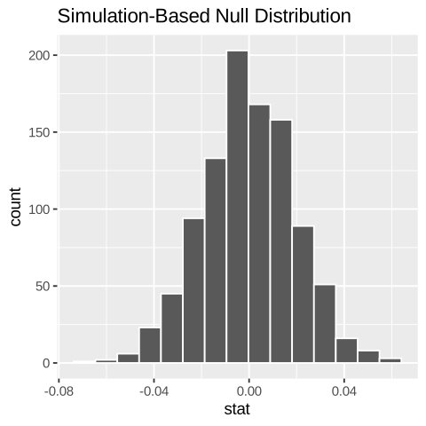
visualize(null_world)

3: Look at δ in the null world

visualize(null_world) +
  shade_p_value(obs_stat = obs_diff, direction = NULL)
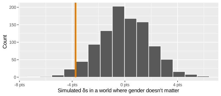
3: Look at δ in the null world

visualize(null_world) +
  shade_p_value(obs_stat = obs_diff, direction = "two-sided")
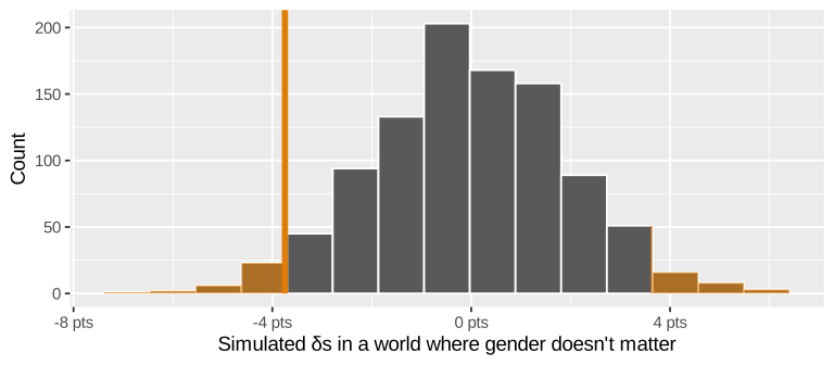
4: Find the p-value

Probability of seeing a δ at least as extreme as ours in this null world

null_world |>
  get_p_value(obs_stat = obs_diff, direction = "two-sided")
# A tibble: 1 × 1
  p_value
    <dbl>
1   0.064

In a world where Lebanese women and men think about emigrating at the same rate, there’s a 6.4% chance that we’d see a difference at least as big as 3.7 percentage points

5: Decide!

p = 0.064

Do we have enough evidence to say that we don’t live in the null world (i.e. to “convict”, or to “reject the null hypothesis”)?

  • Is that below α = 0.05?
  • Is that below α = 0.10?
  • Is that below α = 0.01?

andhs.co/nullworlds

p-values and confidence intervals

lebanon |>
  specify(
    thought_emigrating ~ gender,
    success = "Yes"
  ) |>
  generate(
    reps = 1000,
    type = "bootstrap"
  ) |>
  calculate(
    stat = "diff in props",
    order = c("Female", "Male")
  ) |>
  get_ci(level = 0.95)
lower_ci upper_ci
-0.076 0.0012

The 95% confidence interval includes 0

p is above 0.05

KINDA SORTA SHORTCUT: If a 95% CI includes 0, p > 0.05; if it excludes 0, p < 0.05

thought_emigrating ~ gender

thought_emigrating ~ uses_internet
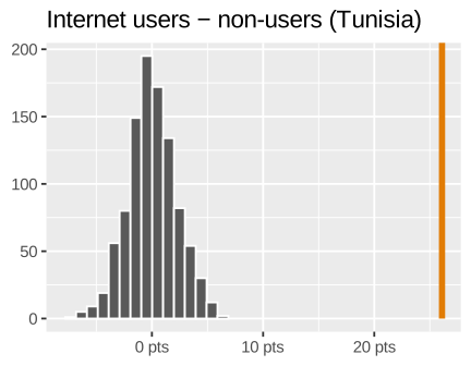
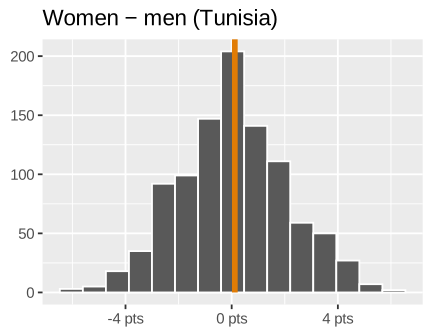
δ = 0.1 points; p ≈ 1

Totally normal in the null world

δ = 26.1 points; p < 0.001

Way off the chart!

Our turn: test some hypotheses

Open hypothesis-testing.qmd in the project

  1. Pick a country and a yes/no question and a comparison group
  2. Write down H_0, H_A, and α before we look at the data
  3. Go through all 5 steps
  4. Interpret results

Diagram of the one test: collected data gives a test statistic δ; simulated data gives a null world of many δs; the p-value is the fraction of simulated δs that exceed the observed δ

  1. Find δ
  2. Invent a world where δ is null
  3. Look at δ in the null world
  4. Find the probability that δ could exist in the null world
  5. Decide!

Interpreting tests

Only two possible outcomes

Reject H_0

p < α

δ doesn’t fit comfortably in the null world, so we’re pretty sure we’re not in it, so δ is probably not 0

“Statistically significant”

Fail to reject H_0

p ≥ α

δ could plausibly show up in the null world

“Not statistically significant”

Temptations!

If p ≥ α (like p = 0.387), you’ll want to say there’s no difference, or that δ is 0

No! Don’t! Bad!

You never “accept” the null hypothesis!

“We find the defendant innocent”
“We find the defendant not guilty”

If p is really close to α (like p = 0.052), you’ll want to say that δ is almost significant

No! Don’t! Bad!

It’s either “guilty”
or not!

“We find the defendant almost guilty”
“We find the defendant not guilty”

The p-value template

In a world where there is no δ, the probability of seeing a δ at least as extreme as ours is p

Then you judge if p is below your evidentiary threshold (0.10, 0.05, 0.01, etc.)

Which is right?

A study finds that a 5-point difference has p = 0.032.

A. There’s a 3.2% chance that the difference is just random

B. There’s a 3.2% chance that our hypothesis is wrong

C. In a world where there’s no difference, there’s a 3.2% chance of seeing a difference at least as extreme as 5 points. That’s below 0.05, so we say it’s statistically significant and reject the null.

C! A p-value is about the data in a null world, not about whether your hypothesis is true

In Lebanon, women are 3.7 points less likely than men to have thought about emigrating (p = 0.064).

A. There’s a 6.4% chance that the null hypothesis is true

B. If there were no gender gap among all Lebanese adults, we’d see a gap at least this big in about 6.4% of samples

C. Since p > 0.05, we’ve shown that Lebanese women and men think about emigrating at the same rate

D. With α = 0.10, we’d reject the null hypothesis

B and D! C is “accepting” the null

Choosing a threshold

  • Smaller α → fewer false positives, but more false negatives
  • Bigger α → fewer false negatives, but more false positives
  • Pick it before you see the data, based on how bad each mistake would be

Everyone uses 0.05, but it’s not magical!

Other δs

Difference in proportions

Do Kuwaiti women and men think about emigrating at different rates?

H_0: p_\text{women} - p_\text{men} = 0

null_world <- kuwait |>
  specify(
    thought_emigrating ~ gender,
    success = "Yes"
  ) |>
  hypothesize(null = "independence") |>
  generate(reps = 1000, type = "permute") |>
  calculate(
    stat = "diff in props",
    order = c("Female", "Male")
  )
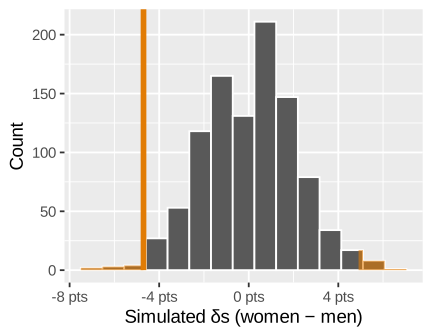
δ = -4.7 points; p = 0.018

Difference in means

Do people in cities and rural areas have different average ages?

H_0: \mu_\text{urban} - \mu_\text{rural} = 0

null_world <- urban_rural |>
  specify(age ~ urban_rural) |>
  hypothesize(null = "independence") |>
  generate(reps = 1000, type = "permute") |>
  calculate(
    stat = "diff in means",
    order = c("Urban", "Rural")
  )
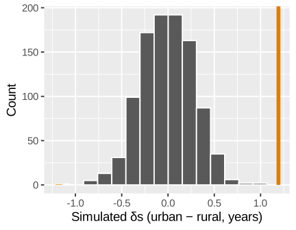
δ = 1.2 years; p < 0.001

One proportion

About 67% of the world used the internet in 2023. Is Tunisia different from the rest of the world?

H_0: p_\text{internet} = 0.67

null_world <- tunisia |>
  drop_na(uses_internet) |>
  specify(
    response = uses_internet,
    success = "Yes"
  ) |>
  hypothesize(null = "point", p = 0.67) |>
  generate(reps = 1000, type = "draw") |>
  calculate(stat = "prop")
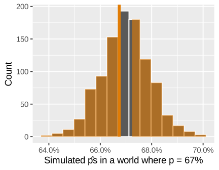
\widehat{p} = 66.7%; p = 0.790

Regression slope

Are older Tunisians less likely to have thought about emigrating?

H_0: \beta_1 = 0

null_world <- tun_ages |>
  specify(yes_num ~ age) |>
  hypothesize(null = "independence") |>
  generate(reps = 1000, type = "permute") |>
  calculate(stat = "slope")
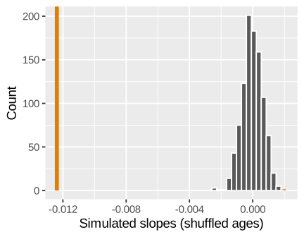
b_1 = -0.0124; p < 0.001
Same general code

Difference in proportions Difference in means One proportion One mean Regression slope
specify() y ~ group,
success = "Yes"
y ~ group response = y,
success = "Yes"
response = y y ~ x
hypothesize() null =
"independence"
null =
"independence"
null = "point",
p = 0.67
null = "point",
mu = 40
null =
"independence"
generate() type =
"permute"
type =
"permute"
type =
"draw"
type =
"bootstrap"
type =
"permute"
calculate() stat =
"diff in props"
stat =
"diff in means"
stat =
"prop"
stat =
"mean"
stat =
"slope"

Math-based tests

Do I have to simulate everything?

No!

  • Math-based tests assume the null world has a known shape (normal, t, χ²)
  • (All those flowcharts and tables are for choosing the right flavor of math-based null world)

Same intuition:
how weird is δ in a world where it’s 0?

Simulation vs. math

lebanon |>
  prop_test(
    thought_emigrating ~ gender,
    success = "Yes",
    order = c("Female", "Male")
  )
Method p
Simulation (1,000 shuffles) 0.064
Math (χ² test) 0.059

Basically the same answer!

Difference in means with t-tests

Do people in cities and rural areas have different average ages?

urban_rural |>
  t_test(
    age ~ urban_rural,
    order = c("Urban", "Rural"),
    alternative = "two-sided"
  )
estimate lower_ci upper_ci statistic p_value
1.19 0.64 1.75 4.24 2.31e-05
  • statistic: how many standard errors δ is away from 0
  • p_value: the probability of seeing that in the null world
  • lower_ci and upper_ci: the 95% confidence interval

Slopes

model <- lm(yes_num ~ age, data = tun_ages)
get_regression_table(model)
term estimate std_error statistic p_value lower_ci upper_ci
intercept 0.9755 0.0275 35.5153 0 0.9217 1.0294
age -0.0124 0.0006 -21.2940 0 -0.0135 -0.0112
  • Every row is a hypothesis test with H_0: \beta = 0
  • statistic is a t statistic, and p_value comes from a t distribution
  • A p_value of 0 isn’t really 0; it’s just super tiny (report it as p < 0.001)
  • Shuffling ages 1,000 times: none of the simulated slopes get anywhere near -0.0124

Build intuition

Even if you never simulate a p-value again, thinking about null worlds is valuable!

Every math-based p-value you see still measures the same thing: how surprising would this δ be in a world where it’s actually 0?

Problems
with p-values

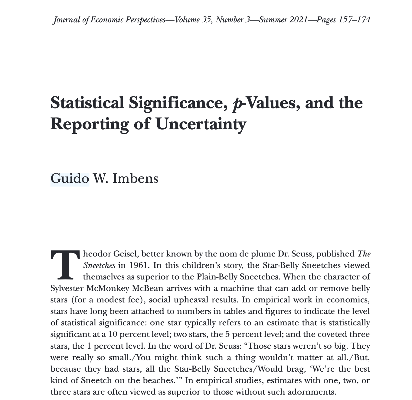
First page of Guido Imbens, 'Statistical Significance, p-Values, and the Reporting of Uncertainty,' Journal of Economic Perspectives 2021, which opens by comparing significance stars to Dr. Seuss's Star-Belly Sneetches

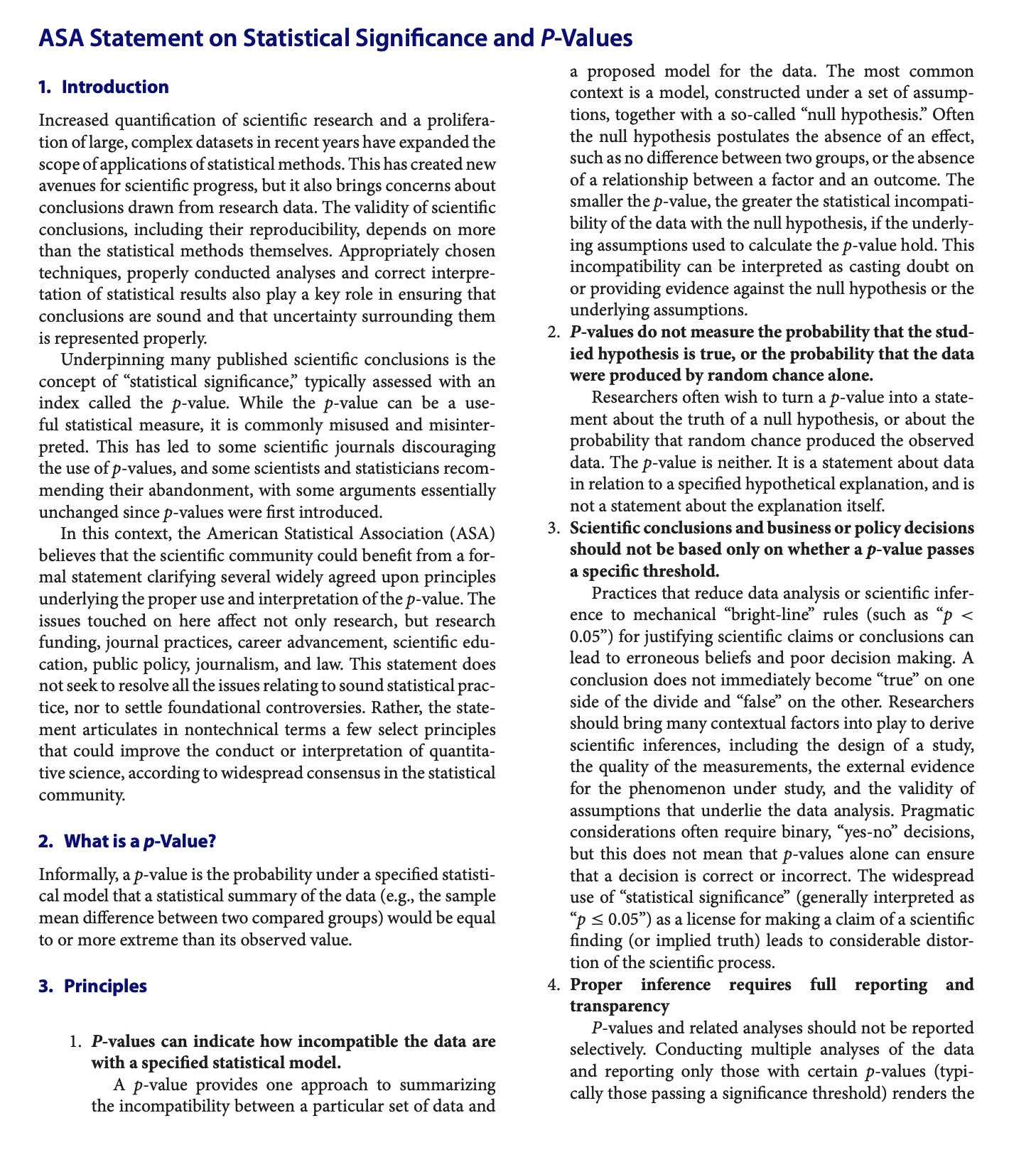
First page of the American Statistical Association's 2016 Statement on Statistical Significance and P-Values

Significant ≠ substantive

Lives in Average age n
Rural 38.5 3,702
Urban 39.7 10,342
  • δ = 1.2 years; p < 0.001
  • Super statistically significant!
  • But does a 1-year age gap matter for anything?
  • With ~14,000 people, even tiny differences become “significant”

Is δ real? Use stats. Does δ matter? That’s up to you!

Do you even need a test?

  • 2,400 people and a 26-point gap. Nobody needs a p-value for this!
  • Look at your data before you run tests

p-hacking

Test enough things and something will be significant

xkcd #882, “Significant”

“Hack Your Way To Scientific Glory”

Decide on your hypotheses and α before you look at the data, and report everything you tested

Preregistration