Inference for regression
Quantitative Methods for
International Politics
IPOL 3270 • Fall 2026
November 15, 2026

Plan for this week
Finish hypothesis testing
Regression and inference
Everything is regression
Reading regression tables
Lots and lots of practice
Leftovers from last week
Regression
and inference
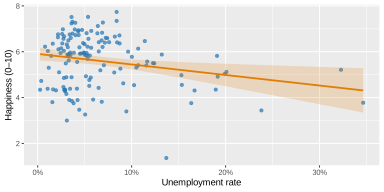
Are countries with higher unemployment less happy?
Slopes are δs too
Are countries with higher unemployment less happy?
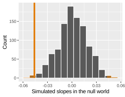
Slopes are δs too
| term | estimate | std_error | statistic | p_value | lower_ci | upper_ci |
|---|---|---|---|---|---|---|
| intercept | 5.905 | 0.146 | 40.555 | 0.000 | 5.617 | 6.193 |
| unemployment_rate | -0.046 | 0.017 | -2.691 | 0.008 | -0.080 | -0.012 |
- Same δ: -0.046
- Basically the same p-value: 0.008 (math) vs. 0.012 (simulation)
- Every row in a regression table is a hypothesis test with H_0: \beta = 0
| term | estimate | std_error | statistic | p_value | lower_ci | upper_ci |
|---|---|---|---|---|---|---|
| intercept | 5.905 | 0.146 | 40.555 | 0.000 | 5.617 | 6.193 |
| unemployment_rate | -0.046 | 0.017 | -2.691 | 0.008 | -0.080 | -0.012 |
| Column | What it means |
|---|---|
estimate |
δ (or β): the slope or the difference between groups |
std_error |
How much the estimate would bounce around from sample to sample |
statistic |
estimate / std_error: how many standard errors δ is away from 0 (a t statistic) |
p_value |
In a world where β is 0ish, the probability of seeing something at least this extreme |
lower_ci, upper_ci |
The 95% confidence interval for β |
Kinda cheating, rough shortcuts
If statistic is bigger than ≈2 (or smaller than ≈−2), p < 0.05
If the 95% confidence interval doesn’t include 0, p < 0.05
Both mean the same thing!
δ is far enough away from 0 that it’d be weird in the null world
Templates
| X | β | p < α | p ≥ α |
|---|---|---|---|
| Continuous | On average, a one-unit increase in X is associated with a β change in Y (confidence interval). | This is statistically significant (p = BLAH), so we are confident that it’s not zero and that there is a relationship. | However, this is not statistically significant (p = BLAH), so we cannot rule out the possibility that the true relationship is zero. |
| Categorical | On average, Y is β higher (or lower) in this group (confidence interval), compared to the base case. | This is statistically significant (p = BLAH), so we are confident that it’s not zero and that there is a difference. | However, this is not statistically significant (p = BLAH), so we cannot rule out the possibility that the true difference is zero. |
| term | estimate | std_error | statistic | p_value | lower_ci | upper_ci |
|---|---|---|---|---|---|---|
| intercept | 5.905 | 0.146 | 40.555 | 0.000 | 5.617 | 6.193 |
| unemployment_rate | -0.046 | 0.017 | -2.691 | 0.008 | -0.080 | -0.012 |
On average, a 1 percentage point increase in the unemployment rate is associated with a 0.046-point decrease in happiness (95% CI: [-0.08, -0.012]). This is statistically significant (p = 0.008), so we are confident that it’s not zero and that there is a relationship.
Is that big? Happiness is on a 0–10 scale, and going from 5% to 15% unemployment would mean happiness drops by about half a point
Everything
is regression
| Test | Question | lm() |
|---|---|---|
| One-sample t-test | Is the average different from 0? | lm(y ~ 1) |
| Two-sample t-test | Are two averages different? | lm(y ~ group_binary) |
| Difference in proportions | Are two proportions different? | lm(y_binary ~ group) |
| ANOVA | Are several averages different? | lm(y ~ category) |
| Multiple regression | All of that ↑, holding other things constant | lm(y ~ x + z + ...) |
Difference in means
Do democracies have higher life expectancy than autocracies?
| Method | δ | p-value |
|---|---|---|
| Simulation (1,000 shuffles) | 7.01 | < 0.001 |
| t-test | 7.01 | < 0.001 |
| Regression | 7.01 | < 0.001 |
Difference in means
Do democracies have higher turnout than autocracies?
| Method | δ | p-value |
|---|---|---|
| Simulation (1,000 shuffles) | 3.26 | 0.272 |
| t-test | 3.26 | 0.232 |
| Regression | 3.26 | 0.232 |
Difference in proportions
Do women and men in Mauritania vote at different rates?
| Method | δ | p-value |
|---|---|---|
| Simulation (1,000 shuffles) | -0.059 | 0.036 |
| Proportion test | -0.059 | 0.032 |
| Regression | -0.059 | 0.032 |
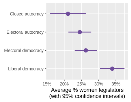
Lots of groups
Women in legislatures across regime types
Holding things constant
Each coefficient in a multiple regression is its own test too
- H_0: β = 0, holding all the other variables constant
- A variable can be significant on its own but stop being significant once you control for other things (or the other way around!)
Our turn: lots of regressions
Open regression-inference.qmd in the project
Reading
regression tables
You’ll see these everywhere
Do richer countries have more women in their legislatures?
| (1) | (2) | (3) | |
|---|---|---|---|
| + p < 0.1, * p < 0.05, ** p < 0.01, *** p < 0.001 | |||
| GDP per capita | 0.092* | 0.046 | |
| (0.036) | (0.038) | ||
| Democracy | 14.128*** | 12.261** | |
| (3.626) | (3.935) | ||
| Constant | 24.016*** | 19.103*** | 18.849*** |
| (1.341) | (2.103) | (2.110) | |
| Num.Obs. | 161 | 161 | 161 |
| R2 | 0.040 | 0.087 | 0.096 |
| (1) | (2) | (3) | |
|---|---|---|---|
| + p < 0.1, * p < 0.05, ** p < 0.01, *** p < 0.001 | |||
| GDP per capita | 0.092* | 0.046 | |
| (0.036) | (0.038) | ||
| Democracy | 14.128*** | 12.261** | |
| (3.626) | (3.935) | ||
| Constant | 24.016*** | 19.103*** | 18.849*** |
| (1.341) | (2.103) | (2.110) | |
| Num.Obs. | 161 | 161 | 161 |
| R2 | 0.040 | 0.087 | 0.096 |
- Each column is a different model
- Each row is a variable
- The number is β
- The number in parentheses underneath is (usually) the standard error
- Stars show the p-value
- An empty cell means that variable isn’t in that model
- The bottom rows describe the whole model: number of observations, R², etc.
| (1) | (2) | (3) | |
|---|---|---|---|
| + p < 0.1, * p < 0.05, ** p < 0.01, *** p < 0.001 | |||
| GDP per capita | 0.092* | 0.046 | |
| (0.036) | (0.038) | ||
| Democracy | 14.128*** | 12.261** | |
| (3.626) | (3.935) | ||
| Constant | 24.016*** | 19.103*** | 18.849*** |
| (1.341) | (2.103) | (2.110) | |
| Num.Obs. | 161 | 161 | 161 |
| R2 | 0.040 | 0.087 | 0.096 |
- Model 1: A $1,000 increase in GDP per capita is associated with 0.092 more percentage points of women legislators, on average (p = 0.011)
- Model 3: Holding democracy constant, that drops to 0.046 and isn’t significant anymore (p = 0.227)
- Democracy stays significant, even after holding wealth constant
- Richer countries tend to be more democratic, so model 1 was partly picking up democracy
Watch out!
- The (parentheses) might be standard errors, t statistics, or p-values, and sometimes [brackets] are confidence intervals
- The stars aren’t standard!
Lots of papers use*p < 0.1,**p < 0.05,***p < 0.01 - Always read the note at the bottom!
library(modelsummary)

model1 <- lm(women_legislators ~ gdp_1000, data = vdem)
model2 <- lm(women_legislators ~ polyarchy, data = vdem)
model3 <- lm(women_legislators ~ gdp_1000 + polyarchy, data = vdem)

modelsummary(
  list("(1)" = model1, "(2)" = model2, "(3)" = model3),
  stars = TRUE,
  gof_map = c("nobs", "r.squared")
)
Use coef_rename or coef_map to give the variables nicer names
Our turn: side-by-side tables
Go to Part 3 in regression-inference.qmd