world_happiness
## # A tibble: 145 × 14
## country year continent region income_group iso3c happiness life_expectancy
## <chr> <dbl> <chr> <chr> <chr> <chr> <dbl> <dbl>
## 1 Finland 2024 Europe Europ… High income FIN 7.74 82.3
## 2 Denmark 2024 Europe Europ… High income DNK 7.52 82.3
## 3 Iceland 2024 Europe Europ… High income ISL 7.52 82.8
## 4 Sweden 2024 Europe Europ… High income SWE 7.34 84.1
## 5 Netherla… 2024 Europe Europ… High income NLD 7.31 82.0
## 6 Costa Ri… 2024 Americas Latin… High income CRI 7.27 81.0
## 7 Norway 2024 Europe Europ… High income NOR 7.26 83.2
## 8 Israel 2024 Asia Middl… High income ISR 7.23 83.2
## 9 Luxembou… 2024 Europe Europ… High income LUX 7.12 83.2
## 10 Mexico 2024 Americas Latin… Upper middl… MEX 6.98 75.3
## # ℹ 135 more rows
## # ℹ 6 more variables: gdp_per_cap <dbl>, internet_use_prop <dbl>,
## # urban_prop <dbl>, women_parliament_prop <dbl>, unemployment_rate <dbl>,
## # population_millions <dbl>Multiple regression I
Readings
- Chester Ismay, Albert Y. Kim, and Arturo Valdivia, Statistical Inference via Data Science: A ModernDive into R and the Tidyverse, 2nd ed. (Chapman and Hall/CRC, 2025), https://doi.org/10.1201/9781032724546, 6.1
- David Diez, Mine Çetinkaya-Rundel, and Christopher D. Barr, OpenIntro Statistics, 4th ed. (OpenIntro, 2019), https://www.openintro.org/book/os/, 9.1–9.2. This one is more mathy than ModernDive—skim it!
- OpenIntro, “Introduction to Multiple Regression”, https://www.youtube.com/watch?v=sQpAuyfEYZg
Slides
Open slides in new window Download PDF of slides
Materials for class today
- Regression playground
.zipproject - Posit.cloud project (only if you’re using an iPad!)
In-class examples
Here’s the code from the two “Our Turn”s and “Your Turns”s from class today. The CSV file of the data is in the .zip file that you downloaded above, or you can grab if from here:
If you’re curious about how I made this data, you can see the R code I used to build, combine, and clean the data here:
library(tidyverse)   # For ggplot, dplyr, and friends
library(moderndive)  # For get_correlation(), get_regression_table(), etc

# Load the World Happiness Report data and only keep 2024
world_happiness <- read_csv("data/world_happiness.csv") |>
  filter(year == 2024)
World happiness
This data comes from the World Happiness Report (happiness scores) and the World Bank (everything else). Each row is a country in 2024.
country: Country nameyear: Yearcontinent: Africa, Americas, Asia, Europe, or Oceaniaregion: World Bank region (East Asia & Pacific, Sub-Saharan Africa, etc.)income_group: World Bank income group (Low income, Lower middle income, Upper middle income, High income)iso3c: Three-letter country codehappiness: Average life evaluation score, on a scale of 0–10 (higher = happier)life_expectancy: Average life expectancy at birth, in yearsgdp_per_cap: GDP per capita (constant 2015 US dollars)internet_use_prop: Percent of the population that uses the internet (0–100)urban_prop: Percent of the population that lives in cities (0–100)women_parliament_prop: Percent of seats in the national parliament held by women (0–100)unemployment_rate: Percent of the labor force that is unemployed (0–100)population_millions: Population, in millions
Our turn #1: Happiness and life expectancy
Does a country’s life expectancy predict its happiness?
Make a scatterplot with life_expectancy on the x-axis and happiness on the y-axis:
ggplot(world_happiness, aes(x = life_expectancy, y = happiness)) +
  geom_point() +
  geom_smooth(method = "lm")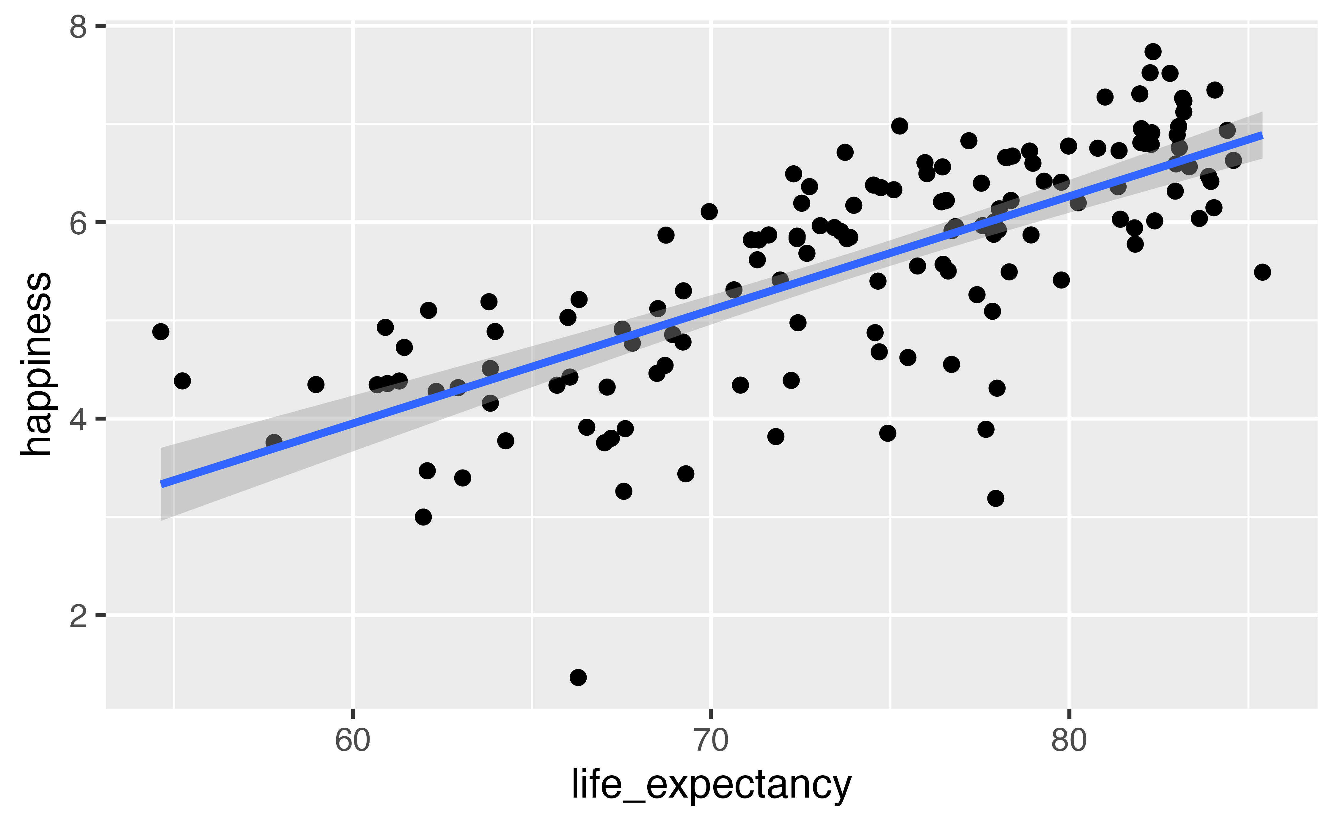
Find the correlation between the two with get_correlation():
get_correlation(world_happiness, happiness ~ life_expectancy)
## # A tibble: 1 × 1
##     cor
##   <dbl>
## 1 0.730
Fit a model with lm() and look at the coefficients with get_regression_table():
model_life_exp <- lm(
  happiness ~ life_expectancy,
  data = world_happiness
)

get_regression_table(model_life_exp)
## # A tibble: 2 × 7
##   term            estimate std_error statistic p_value lower_ci upper_ci
##   <chr>              <dbl>     <dbl>     <dbl>   <dbl>    <dbl>    <dbl>
## 1 intercept         -2.99      0.675     -4.43       0   -4.32    -1.65
## 2 life_expectancy    0.116     0.009     12.8        0    0.098    0.134
Interpret the slope:
On average, a one-year increase in life expectancy is associated with a 0.116 increase in happiness points.
Interpret the intercept:
In a country where life expectancy is 0 years (which doesn’t exist!), average happiness is -2.99.
Your turn #1: Happiness and internet access
Does access to the internet predict national happiness?
Make a scatterplot with internet_use_prop on the x-axis and happiness on the y-axis:
ggplot(data = world_happiness, aes(x = internet_use_prop, y = happiness)) +
  geom_point() +
  geom_smooth(method = "lm")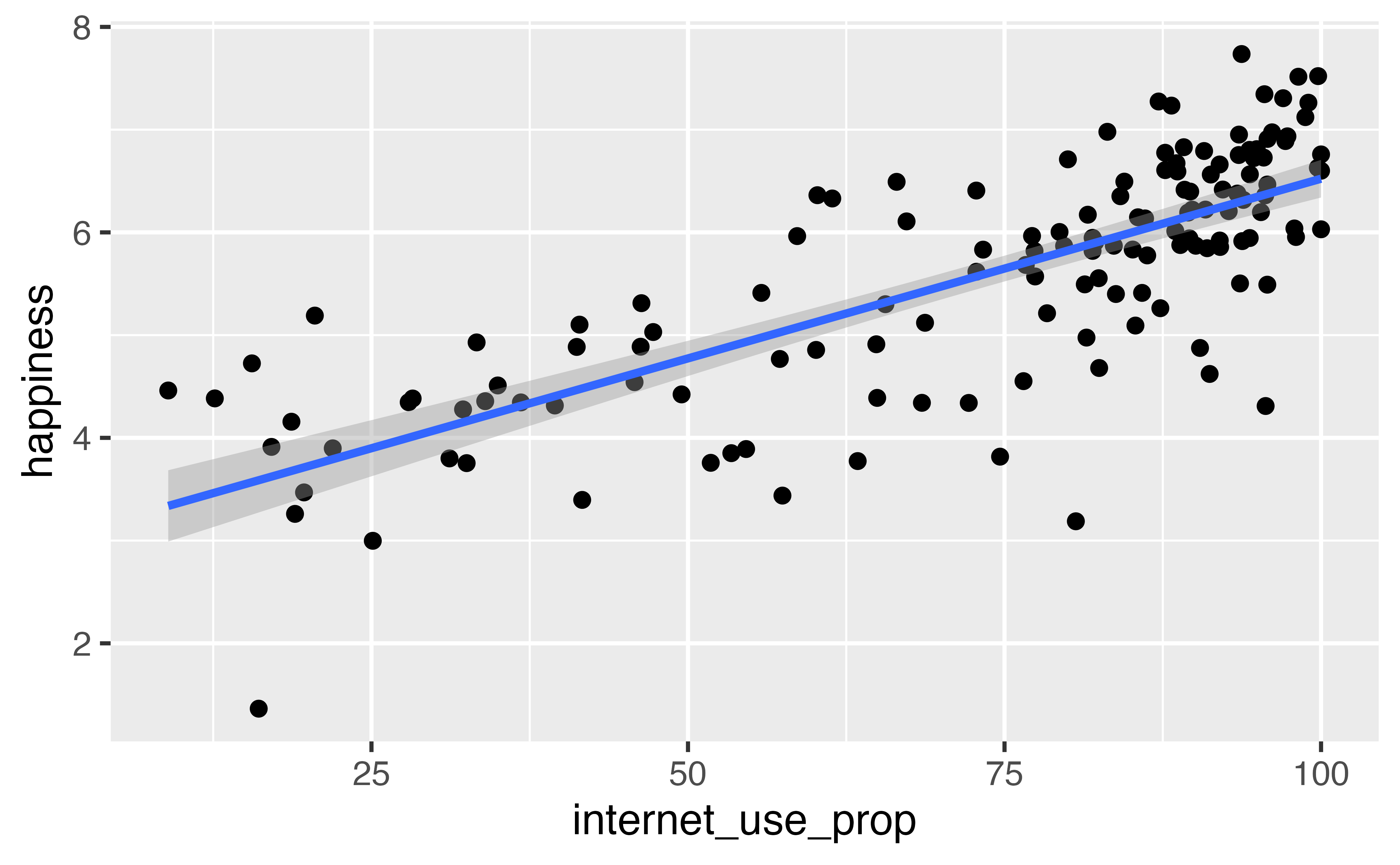
Find the correlation between the two with get_correlation():
get_correlation(world_happiness, happiness ~ internet_use_prop, na.rm = TRUE)
## # A tibble: 1 × 1
##     cor
##   <dbl>
## 1 0.758
Fit a model with lm() and look at the coefficients with get_regression_table():
model_internet <- lm(
  happiness ~ internet_use_prop,
  data = world_happiness
)

get_regression_table(model_internet)
## # A tibble: 2 × 7
##   term              estimate std_error statistic p_value lower_ci upper_ci
##   <chr>                <dbl>     <dbl>     <dbl>   <dbl>    <dbl>    <dbl>
## 1 intercept            3.02      0.197      15.4       0     2.64     3.41
## 2 internet_use_prop    0.035     0.003      13.8       0     0.03     0.04
Interpret the slope:
On average, a one percentage point increase in internet use is associated with a 0.035 point increase in happiness.
Interpret the intercept:
In a country where the proportion of people with access to the internet is 0% (which is potentially plausible!), average happiness is 3.02.
Our turn #2: Happiness and continents
Is happiness different across continents?
Make a plot that shows happiness across each continent (try geom_point() with position = position_jitter(width = 0.15), or geom_boxplot()):
ggplot(data = world_happiness, aes(x = continent, y = happiness)) +
  geom_point(position = position_jitter(width = 0.15))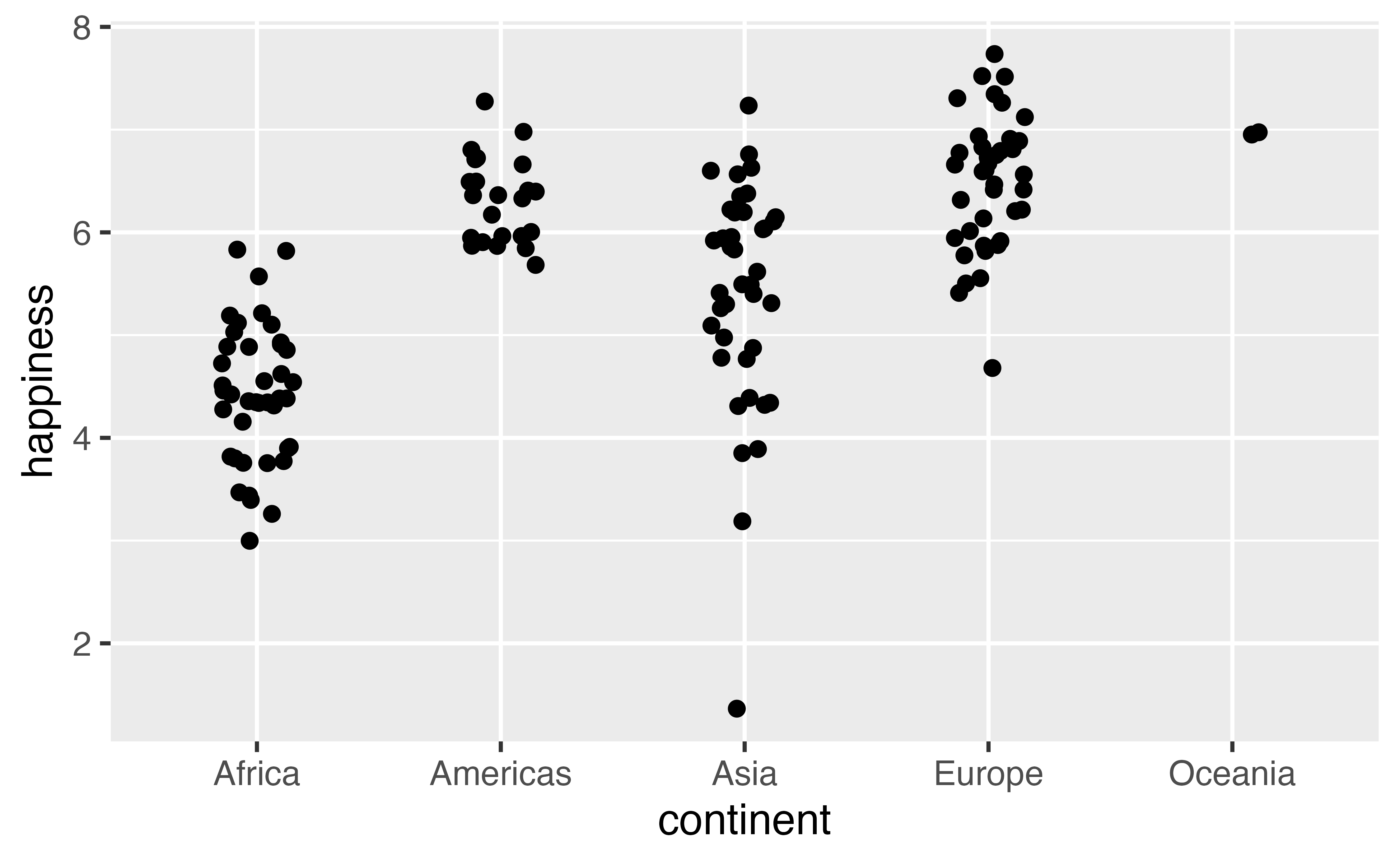
Find the average happiness in each continent with group_by() and summarise():
world_happiness |>
  group_by(continent) |>
  summarise(avg_happiness = mean(happiness))
## # A tibble: 5 × 2
##   continent avg_happiness
##   <chr>             <dbl>
## 1 Africa             4.42
## 2 Americas           6.31
## 3 Asia               5.41
## 4 Europe             6.48
## 5 Oceania            6.96
Fit a model with lm() and look at the coefficients with get_regression_table():
model_happiness_continent <- lm(
  happiness ~ continent,
  data = world_happiness
)

get_regression_table(model_happiness_continent)
## # A tibble: 5 × 7
##   term               estimate std_error statistic p_value lower_ci upper_ci
##   <chr>                 <dbl>     <dbl>     <dbl>   <dbl>    <dbl>    <dbl>
## 1 intercept             4.42      0.123     36.0        0    4.18      4.67
## 2 continent-Americas    1.89      0.205      9.23       0    1.49      2.30
## 3 continent-Asia        0.986     0.175      5.64       0    0.641     1.33
## 4 continent-Europe      2.06      0.176     11.7        0    1.71      2.41
## 5 continent-Oceania     2.54      0.569      4.46       0    1.41      3.66
What’s the base case?
The base case, or omitted continent, is Africa.
Interpret the intercept:
Average happiness in Africa is 4.42.
Interpret the coefficient for Europe:
On average, happiness in Europe is 2.06 points higher than in Africa.
Your turn #2: Internet access and continents
Is internet access different across continents?
Make a plot that shows internet_use_prop across each continent:
ggplot(data = world_happiness, aes(x = continent, y = internet_use_prop)) +
  geom_point(position = position_jitter(width = 0.15))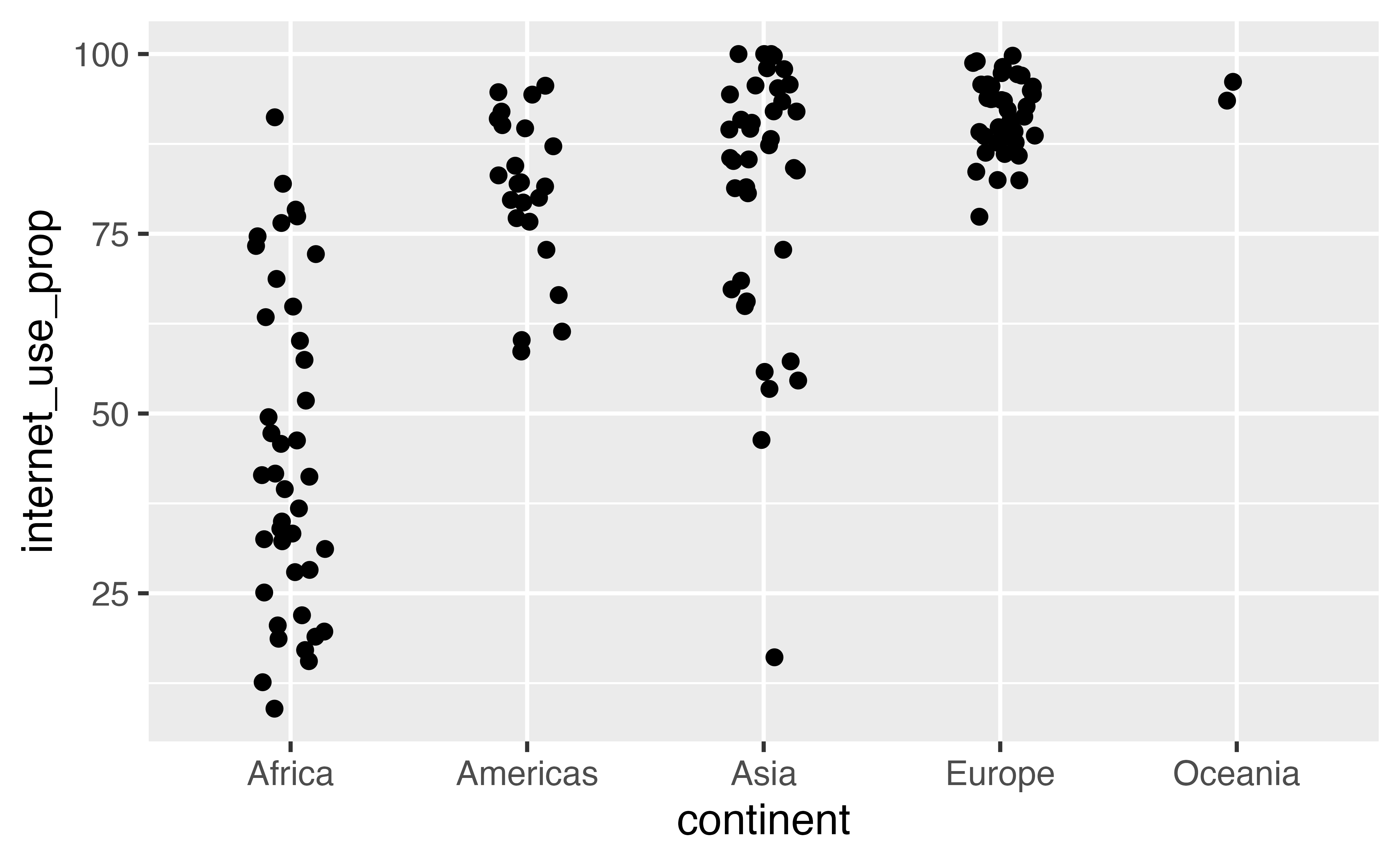
Find the average internet use in each continent with group_by() and summarise():
world_happiness |>
  group_by(continent) |>
  summarise(avg_internet = mean(internet_use_prop, na.rm = TRUE))
## # A tibble: 5 × 2
##   continent avg_internet
##   <chr>            <dbl>
## 1 Africa            44.3
## 2 Americas          80.9
## 3 Asia              81.1
## 4 Europe            91.5
## 5 Oceania           94.8
Fit a model with lm() and look at the coefficients with get_regression_table():
model_internet_continent <- lm(
  internet_use_prop ~ continent,
  data = world_happiness
)

get_regression_table(model_internet_continent)
## # A tibble: 5 × 7
##   term               estimate std_error statistic p_value lower_ci upper_ci
##   <chr>                 <dbl>     <dbl>     <dbl>   <dbl>    <dbl>    <dbl>
## 1 intercept              44.3      2.54     17.4        0     39.2     49.3
## 2 continent-Americas     36.6      4.24      8.64       0     28.2     45.0
## 3 continent-Asia         36.8      3.66     10.0        0     29.5     44.0
## 4 continent-Europe       47.2      3.66     12.9        0     40.0     54.5
## 5 continent-Oceania      50.6     11.8       4.29       0     27.3     73.9
Interpret the intercept:
The average proportion of internet use in Africa is 44.3%.
Interpret the coefficient for Asia:
On average, the proportion of internet use in Asia is 36.8 percentage points higher than in Africa.