world_happiness |>
select(happiness, gdp_per_cap_1000, internet_use_prop) |>
cor(use = "complete.obs")
## happiness gdp_per_cap_1000 internet_use_prop
## happiness 1.0000000 0.6366911 0.7582212
## gdp_per_cap_1000 0.6366911 1.0000000 0.5584973
## internet_use_prop 0.7582212 0.5584973 1.0000000Multiple regression II
Readings
- Chester Ismay, Albert Y. Kim, and Arturo Valdivia, Statistical Inference via Data Science: A ModernDive into R and the Tidyverse, 2nd ed. (Chapman and Hall/CRC, 2025), https://doi.org/10.1201/9781032724546, 6.2–6.3
- David Diez, Mine Çetinkaya-Rundel, and Christopher D. Barr, OpenIntro Statistics, 4th ed. (OpenIntro, 2019), https://www.openintro.org/book/os/, 9.3–9.4. This one is more mathy than ModernDive—again, skim it!
- OpenIntro, “Model Selection in Multiple Regression”, https://www.youtube.com/watch?v=VB1qSwoF-l0
- OpenIntro, “Checking Multiple Regression Diagnostics Using Graphs”, https://www.youtube.com/watch?v=3KSUeYMKt5A
Slides
Open slides in new window Download PDF of slides
Materials for class today
- Multiple regression playground
.zipproject - Posit.cloud project (only if you’re using an iPad!)
In-class examples
Here’s the code from the “We do” and “You do” activities from class today. The CSV file of the data is in the .zip file that you downloaded above, or you can grab if from here:
If you’re curious about how I made this data, you can see the R code I used to build, combine, and clean the data here:
library(tidyverse)   # For ggplot, dplyr, and friends
library(moderndive)  # For get_regression_table(), geom_parallel_slopes(), etc

# Load the World Happiness Report data and only keep 2024
world_happiness <- read_csv("data/world_happiness.csv") |>
  filter(year == 2024) |>
  mutate(
    # GDP per capita in thousands of dollars, so that a "one unit increase" is
    # $1,000 instead of $1
    gdp_per_cap_1000 = gdp_per_cap / 1000,
    # Put the income groups in order (otherwise R puts them in alphabetical order)
    income_group = factor(
      income_group,
      levels = c("Low income", "Lower middle income", "Upper middle income", "High income")
    )
  )
The “I do” example (happiness, life expectancy, urbanization, and region) is already fully worked out in multiple-regression.qmd, so it’s not repeated here.
We do: Happiness, wealth, internet access, and continents
Is national happiness explained by wealth, internet access, and continent?
Use select() and cor() to make a correlation matrix of happiness, gdp_per_cap_1000, and internet_use_prop. A few countries are missing internet_use_prop, so add use = "complete.obs" inside cor() to make it ignore the missing values:
Which variable is more strongly correlated with happiness? How correlated are GDP per capita and internet use with each other?
Internet use is more strongly correlated with happiness (r = 0.76) than GDP per capita is (r = 0.64). GDP per capita and internet use have a correlation of 0.56, which means richer countries tend to have more people online, so some of the explanation they each give for happiness is shared.
Fit a model with lm() that explains happiness with gdp_per_cap_1000, internet_use_prop, and continent, and look at the coefficients with get_regression_table():
model_happiness <- lm(
  happiness ~ gdp_per_cap_1000 + internet_use_prop + continent,
  data = world_happiness
)

get_regression_table(model_happiness)
## # A tibble: 7 × 7
##   term               estimate std_error statistic p_value lower_ci upper_ci
##   <chr>                 <dbl>     <dbl>     <dbl>   <dbl>    <dbl>    <dbl>
## 1 intercept             3.50      0.18     19.5     0        3.15     3.86
## 2 gdp_per_cap_1000      0.015     0.003     4.77    0        0.009    0.022
## 3 internet_use_prop     0.02      0.003     5.73    0        0.013    0.027
## 4 continent-Americas    1.00      0.202     4.96    0        0.602    1.4
## 5 continent-Asia        0.118     0.185     0.641   0.523   -0.247    0.484
## 6 continent-Europe      0.638     0.213     2.99    0.003    0.216    1.06
## 7 continent-Oceania     0.773     0.49      1.58    0.117   -0.196    1.74
What’s the base case for continent?
The base case is Africa, because it’s first alphabetically and it’s the continent that’s missing from the table.
Write out the model as an equation (fill in the numbers):
\[ \begin{aligned} \widehat{\text{happiness}} = &\ 3.50 + 0.015 \times \text{GDP}_{1000} + 0.020 \times \text{internet} + 1.00 \times \text{Americas} \\ &+ 0.12 \times \text{Asia} + 0.64 \times \text{Europe} + 0.77 \times \text{Oceania} \end{aligned} \]
Interpret the intercept:
In an African country with a GDP per capita of $0 and 0% internet use, average happiness would be 3.50 (no country actually has a GDP per capita of $0!).
Interpret the coefficient for GDP per capita:
Controlling for internet use and continent, a $1,000 increase in GDP per capita is associated with a 0.015 point increase in happiness, on average.
Interpret the coefficient for internet use:
Taking GDP per capita and continent into account, a 1 percentage point increase in internet use is associated with a 0.020 point increase in happiness, on average.
Interpret the coefficient for Europe:
Holding GDP per capita and internet use constant, happiness in European countries is 0.64 points higher compared to African countries, on average.
Bonus: plot happiness and gdp_per_cap_1000 with one line for each continent using geom_parallel_slopes(se = FALSE) (this plot ignores internet use, so the lines won’t match the model exactly!):
ggplot(data = world_happiness, aes(x = gdp_per_cap_1000, y = happiness, color = continent)) +
  geom_point() +
  geom_parallel_slopes(se = FALSE)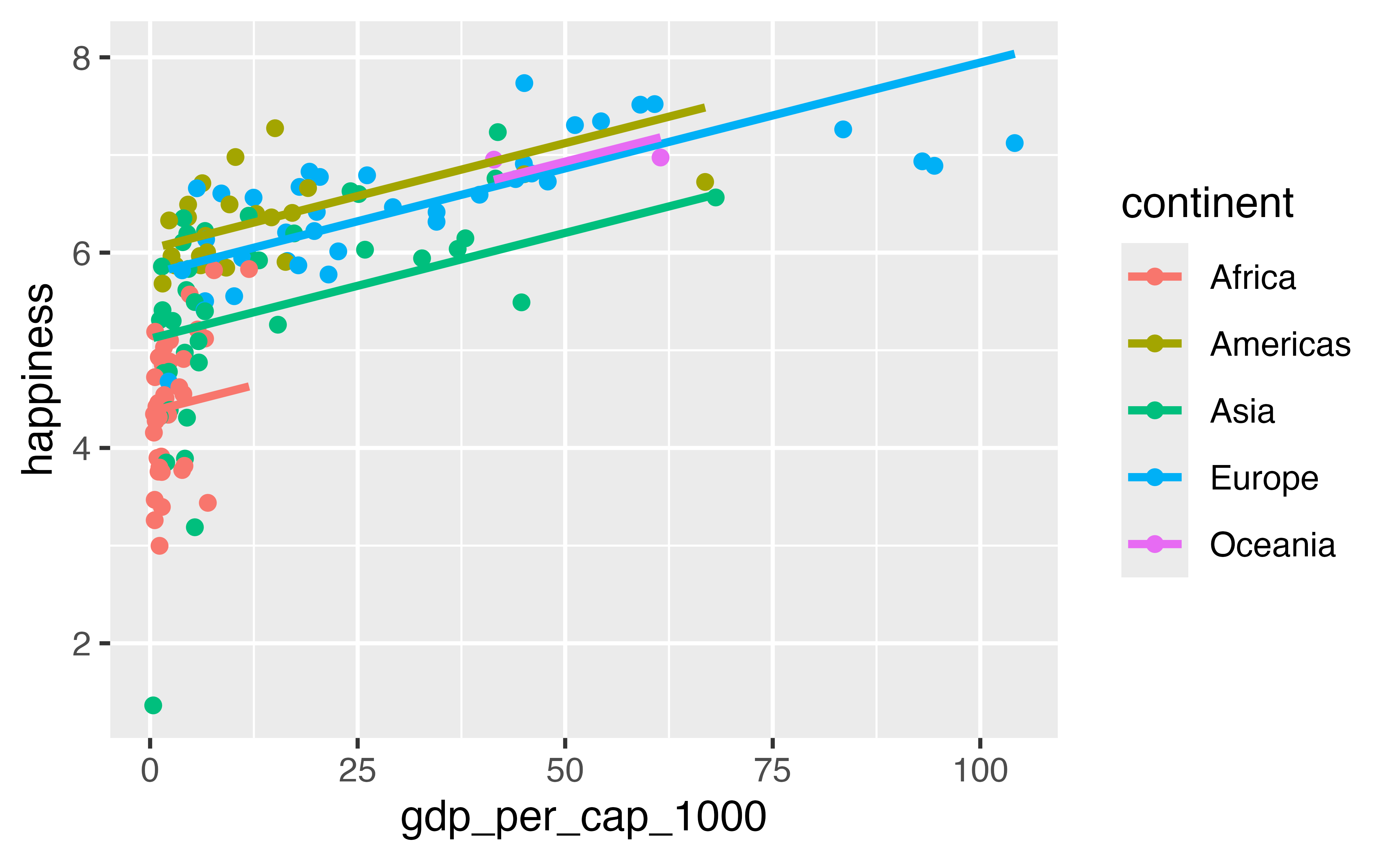
You do together: Happiness, health, jobs, and income
Is national happiness explained by health, jobs, and income?
Make a correlation matrix of happiness, life_expectancy, and unemployment_rate (some countries are missing unemployment_rate, so use use = "complete.obs"):
world_happiness |>
  select(happiness, life_expectancy, unemployment_rate) |>
  cor(use = "complete.obs")
##                    happiness life_expectancy unemployment_rate
## happiness          1.0000000        0.750385        -0.2225016
## life_expectancy    0.7503850        1.000000        -0.1219730
## unemployment_rate -0.2225016       -0.121973         1.0000000
How is happiness related to life expectancy and unemployment? Are life expectancy and unemployment related to each other?
Happiness is strongly and positively correlated with life expectancy (r = 0.75) and weakly and negatively correlated with unemployment (r = −0.22). Life expectancy and unemployment are barely related to each other (r = −0.12), so they’re mostly explaining different parts of the variation in happiness.
Fit a model that explains happiness with life_expectancy, unemployment_rate, and income_group, and look at the coefficients with get_regression_table():
model_income <- lm(
  happiness ~ life_expectancy + unemployment_rate + income_group,
  data = world_happiness
)

get_regression_table(model_income)
## # A tibble: 6 × 7
##   term                    estimate std_error statistic p_value lower_ci upper_ci
##   <chr>                      <dbl>     <dbl>     <dbl>   <dbl>    <dbl>    <dbl>
## 1 intercept                  2.21      0.99       2.23   0.027    0.253    4.17
## 2 life_expectancy            0.031     0.015      2.02   0.045    0.001    0.061
## 3 unemployment_rate         -0.035     0.011     -3.35   0.001   -0.056   -0.014
## 4 income_group-Lower mid…    0.669     0.217      3.08   0.003    0.24     1.10
## 5 income_group-Upper mid…    1.51      0.272      5.55   0        0.973    2.05
## 6 income_group-High inco…    2.05      0.335      6.10   0        1.38     2.71
What’s the base case for income_group, and how do you know?
The base case is “Low income.” It’s not alphabetical (that would be “High income”)—the setup chunk used
factor()to put the income groups in order from lowest to highest, so R uses the first level, “Low income,” as the base case. It’s also the income group that’s missing from the table.
Interpret the coefficient for life expectancy:
Controlling for unemployment and income group, a one-year increase in life expectancy is associated with a 0.031 point increase in happiness, on average.
Interpret the coefficient for unemployment:
Taking life expectancy and income group into account, a 1 percentage point increase in the unemployment rate is associated with a 0.035 point decrease in happiness, on average.
Interpret the coefficient for high income:
Taking life expectancy and unemployment into account, happiness in high income countries is 2.05 points higher than in low income countries, on average.
You do alone: Women in parliament, wealth, and income
Is the share of women in parliament explained by wealth and income group?
Fit a model that explains women_parliament_prop with gdp_per_cap_1000 and income_group, and look at the coefficients with get_regression_table():
model_women <- lm(
  women_parliament_prop ~ gdp_per_cap_1000 + income_group,
  data = world_happiness
)

get_regression_table(model_women)
## # A tibble: 5 × 7
##   term                    estimate std_error statistic p_value lower_ci upper_ci
##   <chr>                      <dbl>     <dbl>     <dbl>   <dbl>    <dbl>    <dbl>
## 1 intercept                 24.8       3.07      8.08    0        18.7     30.9
## 2 gdp_per_cap_1000           0.18      0.066     2.74    0.007     0.05     0.31
## 3 income_group-Lower mid…   -0.554     3.59     -0.155   0.877    -7.65     6.54
## 4 income_group-Upper mid…   -0.07      3.52     -0.02    0.984    -7.02     6.88
## 5 income_group-High inco…   -0.488     4.20     -0.116   0.908    -8.79     7.81
What’s the base case for income_group?
The base case is “Low income,” since the setup chunk put the income groups in order with
factor().
Interpret the coefficient for GDP per capita:
Taking income group into account, a $1,000 increase in GDP per capita is associated with a 0.18 percentage point increase in the share of parliamentary seats held by women, on average.
Interpret the coefficient for one of the income groups:
Taking GDP per capita into account, the share of parliamentary seats held by women in high income countries is 0.49 percentage points lower than in low income countries, on average.
Does anything about these results surprise you?
All the income group coefficients are tiny (less than 1 percentage point) even though high income countries are much richer than low income countries. That’s because GDP per capita and income group measure almost the same thing—the World Bank defines income groups using income per person. Once the GDP slider is in the model, there’s very little left over for the income group switches to explain.